Perfect images of separable metric spaces

Posted on March 28, 2023 by Dan Ma

The Bow-Tie space is the continuous image of a separable metric space and yet is not metrizable (see here). Though taking continuous image can fail to preserve separable metrizability, we show that the perfect image of a separable metric space is a separable metric space. We prove the following theorem, which says that under a perfect map the weight will not increase. The result about separable metric space is a corollary of Theorem 1.

Theorem 1
Let $f:X \longrightarrow Y$ be a perfect map onto the space $Y$ . Then $w(Y) \le w(X)$ , i.e., the weight of $Y$ is no greater than the weight of $X$ .

Proof of Theorem 1

All spaces under consideration are Hausdorff. Let $X$ and $Y$ be spaces. Let $f: \longrightarrow Y$ be a map (or function) from $X$ onto $Y$ . The map $f$ is said to be a closed map if $f(C)$ is closed in $Y$ for any closed subset $C$ of $X$ . The map $f$ is a perfect map if $f$ is continuous, $f$ is a closed map, and $f^{-1}(y)$ is compact for every $y \in Y$ . In words, the last condition is that every point inverse is compact. A point inverse $f^{-1}(y)$ is also referred to as a fiber. Thus, we can say that a perfect map is a continuous closed surjective map with compact fibers. The following lemma is helpful for proving Theorem 1.

Lemma 2
Let $f:X \longrightarrow Y$ be a closed map such that $f(X)=Y$ . Let $V \subset X$ be open. Let $f_*(V)=\{ y \in Y: f^{-1}(y) \subset V \}$ . Then $f_*(V)$ is open in $Y$ and $f_*(V) \subset f(V)$ .

Proof of Lemma 2
We show that $Y \backslash f_*(V)$ is closed in $Y$ . To this end, we show $f(X \backslash V)=Y \backslash f_*(V)$ . Note that $f(X \backslash V)$ is closed in $Y$ since $f$ is a closed map. First, we show $f(X \backslash V) \subset Y \backslash f_*(V)$ . Let $t \in f(X \backslash V)$ . Then $t=f(x)$ for some $x \in X \backslash V$ . Since $x \notin V$ and $x \in f^{-1}(t)$ , we have $f^{-1}(t) \not \subset V$ . This implies that $t \notin f_*(V)$ .

We now show that $Y \backslash f_*(V) \subset f(X \backslash V)$ . Let $z \in Y \backslash f_*(V)$ . Since $z \notin f_*(V)$ , $f^{-1}(z) \not \subset V$ . Choose $x \in f^{-1}(z) \backslash V$ , which implies that $x \in X \backslash V$ . Thus, $z=f(x) \in f(X \backslash V)$ .

To complete the proof of the lemma, we show $f_*(V) \subset f(V)$ . Let $w \in f_*(V)$ . We have $f^{-1}(w) \subset V$ . As a result, $w=f(x)$ for some $x \in V$ . $\square$

Proof of Theorem 1
Let $\mathcal{B}$ be a base for $X$ . We derive a base $\mathcal{B}_1$ for $Y$ such that $\lvert \mathcal{B}_1 \lvert \le \lvert \mathcal{B} \lvert$ , i.e., the cardinality of $\mathcal{B}_1$ is no more than the cardinality of $\mathcal{B}$ . This implies that the minimal cardinality of a base in $Y$ is no more than the minimal cardinality of a base in $X$ , i.e., $w(Y) \le w(X)$ .

We assume that the base $\mathcal{B}$ is closed under finite unions. We show that $\mathcal{B}_1=\{ f_*(B): B \in \mathcal{B} \}$ is a base for $Y$ . Note that $f_*$ is defined in Lemma 2. Let $U \subset Y$ be an open set. Let $y \in U$ . For each $x \in f^{-1}(y)$ , choose $B_x \in \mathcal{B}$ such that $x \in B_x$ and $f(B_x) \subset U$ . Since $f^{-1}(y)$ is compact, there exists finite $F \subset f^{-1}(y)$ such that $f^{-1}(y) \subset \bigcup_{t \in F} B_t=B$ . Note that $B \in \mathcal{B}$ . Since $f^{-1}(y) \subset B$ , we have $y \in f_*(B)$ . We also have $f_*(B) \subset f(B) \subset U$ . Thus, every open subset $U$ of $Y$ is the union of elements of $\mathcal{B}_1$ . This means that $\mathcal{B}_1$ is a base for $Y$ . Theorem 1 is established. $\square$

Corollary 3
Let $f:X \longrightarrow Y$ be a perfect map onto the space $Y$ . Then if $X$ is a separable metric space, then $Y$ is a separable metric space.

Comment About Lemma 2
A perfect map is not necessarily an open map. If the perfect map $f$ in Theorem 1 is an open map, then Lemma 2 is not needed and $\mathcal{B}_1=\{ f(B): B \in \mathcal{B} \}$ would be a base for $Y$ . However, we cannot assume $f$ is an open map simply because it is a perfect map. To see this, let $X=\mathbb{R}$ be the real line with the usual topology. Collapse the closed interval $[1,2]$ to one point called $p$ . The resulting quotient space is $Y$ where $Y=(-\infty,1) \cup \{ p \} \cup (2,\infty)$ . In $Y$ , the open neighborhoods of points in $(-\infty,1) \cup (2,\infty)$ are the usual Euclidean neighborhoods. The open neighborhoods of the point $p$ are the usual Euclidean open sets containing the interval $[1,2]$ . The resulting quotient map $f$ is an identity map on $(-\infty,1) \cup (2,\infty)$ and it maps points in $[1,2]$ to the point $p$ . It can be verified that $f$ is a perfect map. For the open set $V=(1,2)$ , $f(V)=\{ p \}$ , which is not open in $Y$ . For the open set $V=(0,1.5)$ , $f(V)=(0,1) \cup \{ p \}$ , which is not open in $Y$ . Lemma 2 says that for any open $X \subset$ , $f(V)$ may not be open but has an open subset $f_*(V)$ if $f(V)$ has non-empty interior. The interior sets $f_*(V)$ can work as a base in $Y$ .

Invariant and Inverse Invariant

Let $\mathcal{P}$ be a property of topological spaces. We say that $\mathcal{P}$ is an invariant of the perfect maps or that $\mathcal{P}$ is invariant under the perfect maps if the property $\mathcal{P}$ is preserved by perfect maps, i.e., for each perfect map $f:X \longrightarrow Y$ where $Y=f(X)$ , if the space $X$ has $\mathcal{P}$ , so does $Y$ . On the other hand, $\mathcal{P}$ is an inverse invariant of the perfect maps if this holds: for each perfect map $f:X \longrightarrow Y$ where $Y=f(X)$ , if $Y$ has $\mathcal{P}$ , so does $X$ .

The notions invariant and inverse invariant defined here are for perfect maps. In general, the notions are much broader and can be defined in relation to any class of continuous maps. For example, we know that the continuous image of a separable space is separable. We can say that separability is an invariant of the continuous maps or that separability is invariant under continuous maps. We can now restate Theorem 1 and Corollary 3 as follows.

Theorem 4…..Restatement of Theorem 1
The property “weight $\le \mathcal{K}$ ” is an invariant of the perfect maps.

Corollary 5
The second axiom of countability is invariant under the perfect maps, but is not an invariant of the continuous maps.

The Bow-Tie space is the continuous image of a separable space but cannot have a countable base (see here). In light of Theorem 1, the continuous map that maps a separable metric space to the Bow-Tie space (shown here) cannot be a perfect map. With respect to that map, the upper half plane in the domain (the separable metric space) is closed but its continuous image in the Bow-Tie space is open and not closed.

$\text{ }$

Dan Ma Bow-Tie space
Daniel Ma Bow-Tie space

Dan Ma perfect map
Daniel Ma perfect map

Dan Ma separable metric space
Daniel Ma separable metric space

Dan Ma topology
Daniel Ma topology

$\copyright$ 2023 – Dan Ma

Revised March 31, 2023
Revised March 12, 2024

The Bow-Tie Space

Posted on March 26, 2023 by Dan Ma

We present the Bow-Tie space, which exhibits many interesting properties. The Bow-Tie space is hereditarily Lindelof, and hereditarily separable. It is also the continuous image of a separable metric space. These properties follow from the fact that the Bow-Tie space has a countable network. Furthermore, the Bow-Tie space is neither metrizable nor a Moore space. Thus, the example demonstrates that the continuous image of a separable metric space does not have to be a separable metric space.

Louis F. McAuley introduced the Bow-Tie space as an example of a regular semimetric space that is hereditarily separable, collectionwise normal, completely normal and paracompact, but is not second countable and is not developable, hence not a Moore space [3]. The Bow-Tie space is also discussed in Counterexamples in Topology [5] (see p. 175 Dover Edition). In these two references, the Bow-Tie space is defined as a semimetric space. The version given here is found in [4]. The Bow-Tie space is given in [4] as an example of a cosmic space (i.e., a space with a countable network) that is not an $\aleph_0$ -space.

All spaces under consideration are Hausdorff. Let $X$ be a space. A collection $\mathcal{N}$ of subsets of $X$ is said to be a network for $X$ if for each $x \in X$ and for each open set $O$ containing $x$ , there exists $A \in \mathcal{N}$ such that $x \in A \subset O$ . A network behaves like a base but the elements of the network do not have to be open sets. Of interest are the spaces with a countable network. Compact spaces with a countable network is metrizable. Any space with a countable network is both hereditarily separable and hereditarily Lindelof. The space $X$ has a countable network if and only if $X$ is the continuous image of a separable metric space. Having a countable network is a strong property. See here for a discussion of these facts about spaces with countable network.

The Bow-Tie Space

Let $Y$ be the upper half plane, which is the set of all pairs of real numbers $(x,y)$ with $y>0$ . Let $H$ be the x-axis, which is the set of all pairs of real numbers $(x,y)$ with $y=0$ . The bow-tie space is the set $X=Y \cup H$ with the topology defined as follows.

Open neighborhoods of points in the upper half plane $Y$ are the Euclidean open subsets of $Y$ .
An open neighborhood of a point $p$ in the x-axis $H$ is of the form $B(p,c)$ with $0<c \le 1$ . Each set $B(p,c)$ consists of the point $p$ and all points $q \in X$ having Euclidean distance less than $c$ from $p$ and lying underneath either one of the two straight lines emanating from $p$ with slopes $c$ and $-c$ , respectively.

In the following diagram, $B(p,c)$ is represented by the area in the upper half plane shaded in green plus the points in the x-axis having a distance less than $c$ from $p$ and below the two lines with slopes $c$ and $-c$ .

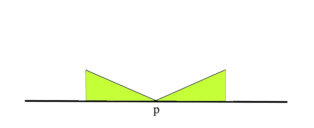
It is straightforward to verify that the open neighborhoods produce a Hausdorff and regular space. The relative Bow-Tie topologies on $Y$ and $H$ coincide with the Euclidean topologies on $Y$ and $H$ , respectively. Let $\mathcal{B}_1$ and $\mathcal{B}_2$ be countable bases for $Y$ and $H$ in their respective relative Euclidean topologies. Then $\mathcal{N}=\mathcal{B}_1 \cup \mathcal{B}_2$ is a network for the Bow-Tie space $X$ . Thus, the Bow-Tie space has a countable network. Any space with a countable network is Lindelof and separable. The property of having a countable netowrk is hereditary. Thus, the Bow-Tie space is hereditarily Lindelof and hereditarily separable. See here for a discussion of these facts about spaces with countable network.

Any space with a countable network is the continuous image of a separable metric space. In the case of the Bow-Tie space, we can see this directly. Let $Y_1$ be the upper half plane $Y$ with the Euclidean topology. Let $H_1$ be the x-axis $H$ with the Euclidean topology. Let $X_1=Y_1 \bigoplus H_1$ , the free sum or free union. This means that $U \subset X_1$ is open if and only if both $U \cap Y_1$ and $U \cap H_1$ are open. It follows that the identity map from $X_1$ onto the Bow-Tie space $X$ is continuous.

The Bow-Tie space $X$ is separable but not metrizable. We show that $X$ does not have a countable base. Suppose it does. Let $\mathcal{B}$ be a countable base for the Bow-Tie space. We can assume that the elements of $\mathcal{B}$ that contain points of the x-axis $H$ are of the form $B(p,c)$ defined above. Since $\mathcal{B}$ is countable, there can only be countably many $B(p,c)$ in $\mathcal{B}$ , say, $B(p_0,c_0)$ , $B(p_1,c_1)$ , $B(p_2,c_2)$ , $B(p_3,c_3),\cdots$ . Pick $p \in H$ such that $p \ne p_i$ for all $i$ . Consider $B(p,1)$ . Since $\mathcal{B}$ is a base, there must exist some $i$ such that $p \in B(p_i,c_i) \subset B(p,1)$ . This means that both the left side and the right side of the bow-tie in $B(p_i,c_i)$ are within $B(p,1)$ . On the other hand, one side of the bow-tie of $B(p_i,c_i)$ (either the left side or the right side) is above the point $p$ . The points on that side of the bow-tie of $B(p_i,c_i)$ right above point $p$ cannot be part of $B(p,1)$ , a contradiction. Thus, the Bow-Tie space $X$ cannot have a countable base and hence not metrizable. The Bow-Tie space cannot be a Moore space since any Lindelof Moore space must have a countable base.

Not only the Bow-Tie space cannot have a countable base, it also cannot have a point-countable base. For any space, a base is a point-countable base if every point in the space belongs to only countably many elements of the base. In [3] and [5], the Bow-Tie space is defined using a semimetric. Heath [2] showed that every semimetric space with a point-countable base is developable, hence a Moore space if the space is regular. The Bow-Tie space cannot have a point-countable base. If it does, it would be a Moore space.

We mention two more facts about the Bow-Tie space. One is that the Bow-Tie space is a Lindelof $\Sigma$ -space. It is well known that any space with a countable network is a Lindelof $\Sigma$ -space [6]. Secondly, $C_p(X)$ , the function space with the pointwise convergence topology on the Bow-Tie space $X$ is a hereditarily D-space. Gruenhage [1] showed that if $L$ is a Lindelof $\Sigma$ -space, then $C_p(L)$ is a hereditarily D-space.

Reference

Gruenhage, G., A note on D-spaces, Topology and Appl. 152, 2229-2240, 2006.
Heath, R. W., On spaces with point-countable bases, Bull. Acad. Polon. Sci. 13, 393-395, 1965.
McAuley, L. F., A relation between perfect separability, completeness, and normality in semimetric spaces, Pacific J. Math. 6, 315-326, 1956.
Michael, E., $\aleph_0$ -spaces, J. Math. Mech., 15, 983-1002, 1966.
Steen, L. A., Seebach, J. A., Counterexamples in Topology, Dover Publications, Inc., New York, 1995.
Tkachuk, V. V., Lindelof $\Sigma$ -spaces: an omnipresent class, RACSAM, 104 (2), 221-244, 2010.

$\text{ }$

Dan Ma Bow-Tie space
Daniel Ma Bow-Tie space

Dan Ma hereditarily Lindelof space
Daniel Ma hereditarily Lindelof space

Dan Ma hereditarily separable space
Daniel Ma hereditarily separable space

Dan Ma countable network
Daniel Ma countable network

Dan Ma topology
Daniel Ma topology

$\copyright$ 2023 – Dan Ma

Spaces With Countable Network

Posted on November 14, 2009 by Dan Ma

The concept of network is a useful tool in working with generalized metric spaces. A network is like a base for a topology, but the members of a network do not have to be open. After a brief discussion on network, the focus here is on the spaces with networks that are countably infinite in size. The following facts are presented:

Any space with a countable network is separable and Lindelof.
The property of having a countable network is hereditary. Thus any space with a countable network is hereditarily separable and hereditarily Lindelof.
The property of having a countable network is preserved by taking countable product.
The Sorgenfrey Line is an example of a hereditarily separable and hereditarily Lindelof space that has no countable network.
For any compact space $X$ , $nw(X)=w(X)$ . In particular, any compact space with a countable network is metrizable.
As a corollary to 5, $w(X) \leq \vert X \vert$ for any compact $X$ .
A space $X$ has a countable network if and only if it is the continuous impage of a separable metric space (hence such a space is sometimes called cosmic).
Any continuous image of a cosmic space is cosmic.
Any continuous image of a compact metric space is a compact metric space.
As a corollary to 2, any space with countable network is perfectly normal.
An example is given to show that the continuous image of a separable metric space needs not be metric (i.e. an example of a cosmic space that is not metrizable).

All spaces in this discussion are at least $T_3$ (Hausdorff and regular). Let $X$ be a space. A collection $\mathcal{N}$ of subsets of $X$ is said to be a network for $X$ if for each $x \in X$ and for each open $U \subset X$ with $x \in U$ , then we have $x \in N \subset U$ for some $N \in \mathcal{N}$ . The network weight of a space $X$ , denoted by $nw(X)$ , is defined as the minimum cardinality of all the possible $\vert \mathcal{N} \vert$ where $\mathcal{N}$ is a network for $X$ . The weight of a space $X$ , denoted by $w(X)$ , is defined as the minimum cardinality of all possible $\vert \mathcal{B} \vert$ where $\mathcal{B}$ is a base for $X$ . Obviously any base is also a network. Thus $nw(X) \leq w(X)$ . For any compact space $X$ , $nw(X)=w(X)$ . On the other hand, the set of singleton sets is a network. Thus $nw(X) \leq \vert X \vert$ .

Our discussion is based on an important observation. Let $\mathcal{T}$ be the topology for the space $X$ . Let $\mathcal{K}=nw(X)$ . We can find a base $\mathcal{B}_0$ that generates a weaker (coarser) topology such that $\lvert \mathcal{B}_0 \lvert=\mathcal{K}$ . We can also find a base $\mathcal{B}_1$ that generates a finer topology such that $\lvert \mathcal{B}_1 \lvert=\mathcal{K}$ . These are restated as lemmas.

Lemma 1. We can define base $\mathcal{B}_0$ that generates a weaker (coarser) topology $\mathcal{S}_0$ on $X$ such that $\lvert \mathcal{B}_0 \lvert=\mathcal{K}$ . Thus $w(X,\mathcal{S}_0) \leq nw(X)$ .

Proof. Let $\mathcal{N}$ be a network for $(X,\mathcal{T})$ such that $\vert \mathcal{N} \vert=nw(X,\mathcal{T})$ . Consider all pairs $N_0,N_1 \in \mathcal{N}$ such that there exist disjoint $O_0,O_1 \in \mathcal{T}$ with $N_0 \subset O_0$ and $N_1 \subset O_1$ . Such pairs exist because we are working in a Hausdorff space. Let $\mathcal{B}_0$ be the collection of all such open sets $O_0,O_1$ and their finite interections. This is a base for a topology and let $\mathcal{S}_0$ be the topology generated by $\mathcal{B}_0$ . Clearly, $\mathcal{S}_0 \subset \mathcal{T}$ and this is a Hausdorff topology. Note that $w(X,\mathcal{S}_0) \leq \vert \mathcal{B}_0 \vert =\vert \mathcal{N} \vert$ .

Lemma 2. We can define base $\mathcal{B}_1$ that generates a finer topology $\mathcal{S}_1$ on $X$ such that $\lvert \mathcal{B}_1 \lvert=\mathcal{K}$ . Thus $w(X,\mathcal{S}_1) \leq nw(X)$ .

Proof. As before, let $\mathcal{N}$ be a network for $(X,\mathcal{T})$ such that $\vert \mathcal{N} \vert=nw(X,\mathcal{T})$ . Since we are working in a regular space, we can assume that the sets in $\mathcal{N}$ are closed. If not, take closures of the elements of $\mathcal{N}$ and we still have a network. Consider $\mathcal{B}_1$ to be the set of all finite intersections of elements in $\mathcal{N}$ . This is a base for a topology on $X$ . Let $\mathcal{S}_1$ be the topology generated by this base. Clearly, $\mathcal{T} \subset \mathcal{S}_1$ . It is also clear that $w(X,\mathcal{S}_1) \leq nw(X)$ . The only thing left to show is that the finer topology is regular. Note that the network $\mathcal{N}$ consists of closed sets in the topology $\mathcal{T}$ . Thus the sets in the base $\mathcal{B}_1$ also consists of closed sets with respect to $\mathcal{T}$ and the sets in $\mathcal{B}_1$ are thus closed in the finer topology. Since $\mathcal{B}_1$ is a base consisting of cloased and open sets, the topology $\mathcal{S}_1$ regular.

Discussion of 1, 2, and 3
Points 1, 2 and 3 are basic facts about countable network and they are easily verified based on definitions. They are called out for the sake of having a record.

Discussion of 4
The Sorgenfrey Line does not have a countable network for the same reason that the Sorgenfrey Plane is not Lindelof. If the Sorgenfrey Line has a countable netowrk, then the Sorgenfrey plane would have a countable network and hence Lindelof.

Discussion of 5
In general, $nw(X) \leq w(X)$ . In a compact Hausdorff space, any weaker Hausdorff topology must conincide with the original topology. So the weaker topology produced in Lemma 1 must coincide with the original topology. In the countable case, any compact space with a countable network has a weaker topology with a countable base. This weaker topology must coincide with the original topology.

Discussion of 6
Note that $nw(X) \leq \lvert X \lvert$ always holds. For compact spaces, we have $w(X)=nw(X) \leq \lvert X \lvert$ .

Discussion of 7
Let $X$ be a space with a countable network. By Lemma 2, $X$ has a finer topology that has a countable base. Let $Y$ denote $X$ with this finer second countable topology. Then the identity map from $Y$ onto $X$ is continuous.

For the other direction, let $f:Y \rightarrow X$ be a continuous function mapping a separable metric space $Y$ onto $X$ . Let $\mathcal{B}$ be a countable base for $Y$ . Then $\lbrace{f(B):B \in \mathcal{B}}\rbrace$ is a network for $X$ .

Discussion of 8
This is easily verified. Let $X$ is the continuous image of a cosmic space $Y$ . Then $Y$ is the continuous image of some separable metric space $Z$ . It follows that $X$ is the continuous image of $Z$ .

Discussion of 9
Let $X$ be compact metrizable and let $Y$ be a continuous image of $X$ . Then $Y$ is compact. By point 7, $Y$ has a countable network. By point 5, $Y$ is metrizable.

Discussion of 10
A space is perfectly normal if it is normal and that every closed subset is a $G_\delta-$ set. Let $X$ be a space with a countable network. The normality of $X$ comes from the fact that it is regular and Lindelof. Note that $X$ is also hereditarily Lindelof. In a hereditarily Lindelof and regular space, every open subspace is an $F_\sigma-$ set (thus every closed set is a $G_\delta-$ set.

Discussion of 11 (Example of cosmic but not separable metrizable space)
This is the “Butterfly” space or “Bow-tie” space due to L. F. McAuley. I found this example in [Michael]. Let $Y=T \cup S$ where
$T=\lbrace{(x,y) \in \mathbb{R}^2:y>0}\rbrace$ and
$S=\lbrace{(x,y) \in \mathbb{R}^2:y=0}\rbrace$ .

Points in $T$ have the usual plane open neighborhoods. A basic open set at $p \in S$ is of the form $B_c(p)$ where $B_c(p)$ consists of $p$ and all points $q \in Y$ having distance $<c$ from $p$ and lying underneath either one of the two straight lines in $Y$ which emanate from $p$ and have slopes $+c$ and $-c$ , respectively.

It is clear that $Y$ is a Hausdorff and regular space. The relative “Bow-tie” topologies on $T$ and $S$ coincide with the usual topology on $T$ and $S$ , respectively. Thus the union of the usual countable bases on $T$ and $S$ would be a countable network for $Y$ . On the other hand, $Y$ is separable but cannot have a countable base (hence not metrizable).

Reference
[Michael]
Michael, E., $\aleph_0-$ spaces, J. Math. Mech. 15, 983-1002.

Dan Ma's Topology Blog

Expository Articles In General Topology

Tag Archives: Bow-tie space

Perfect images of separable metric spaces

The Bow-Tie Space

Spaces With Countable Network