Michael line and Morita’s conjectures

This post discusses Michael line from the point of view of the three conjectures of Kiiti Morita.

K. Morita defined the notion of P-spaces in [7]. The definition of P-spaces is discussed here in considerable details. K. Morita also proved that a space X is a normal P-space if and only if the product X \times Y is normal for every metrizable space Y. As a result of this characterization, the notion of normal P-space (a space that is a normal space and a P-space) is useful in the study of products of normal spaces. Just to be clear, we say a space is a non-normal P-space (i.e. a space that is not a normal P-space) if the space is a normal space that is not a P-space.

K. Morita formulated his three conjectures in 1976. The statements of the conjectures are given below. Here is a basic discussion of the three conjectures. The notion of normal P-spaces is a theme that runs through the three conjectures. The conjectures are actually theorems since 2001 [2].

Here’s where Michael line comes into the discussion. Based on the characterization of normal P-spaces mentioned above, to find a normal space that is not a P-space (a non-normal P-space), we would need to find a non-normal product X \times Y such that one of the factors is a metric space and the other factor is a normal space. The first such example in ZFC is from an article by E. Michael in 1963 (found here and here). In this example, the normal space is M, which came be known as the Michael line, and the metric space is \mathbb{P}, the space of irrational numbers (as a subspace of the real line). Their product M \times \mathbb{P} is not normal. A basic discussion of the Michael line is found here.

Because M \times \mathbb{P} is not normal, the Michael line M is not a normal P-space. Prior to E. Michael’s 1963 article, we have to reach back to 1955 to find an example of a non-normal product where one factor is a metric space. In 1955, M. E. Rudin used a Souslin line to construct a Dowker space, which is a normal space whose product with the closed unit interval is not normal. The existence of a Souslin line was shown to be independent of ZFC in the late 1960s. In 1971, Rudin constructed a Dowker space in ZFC. Thus finding a normal space that is not a normal P-space (finding a non-normal product X \times Y where one factor is a metric space and the other factor is a normal space) is not a trivial matter.

Morita’s Three Conjectures

We show that the Michael line illustrates perfectly the three conjectures of K. Morita. Here’s the statements.

Morita’s Conjecture I. Let X be a space. If the product X \times Y is normal for every normal space Y then X is a discrete space.

Morita’s Conjecture II. Let X be a space. If the product X \times Y is normal for every normal P-space Y then X is a metrizable space.

Morita’s Conjecture III. Let X be a space. If the product X \times Y is normal for every normal countably paracompact space Y then X is a metrizable \sigma-locally compact space.

The contrapositive statement of Morita’s conjecture I is that for any non-discrete space X, there exists a normal space Y such that X \times Y is not normal. Thus any non-discrete space is paired with a normal space for forming a non-normal product. The Michael line M is paired with the space of irrational numbers \mathbb{P}. Obviously, the space \mathbb{P} is paired with the Michael line M.

The contrapositive statement of Morita’s conjecture II is that for any non-metrizable space X, there exists a normal P-space Y such that X \times Y is not normal. The pairing is more specific than for conjecture I. Any non-metrizable space is paired with a normal P-space to form a non-normal product. As illustration, the Michael line M is not metrizable. The space \mathbb{P} of irrational numbers is a metric space and hence a normal P-space. Here, M is paired with \mathbb{P} to form a non-normal product.

The contrapositive statement of Morita’s conjecture III is that for any space X that is not both metrizable and \sigma-locally compact, there exists a normal countably paracompact space Y such that X \times Y is not normal. Note that the space \mathbb{P} is not \sigma-locally compact (see Theorem 4 here). The Michael line M is paracompact and hence normal and countably paracompact. Thus the metric non-\sigma-locally compact \mathbb{P} is paired with normal countably paracompact M to form a non-normal product. Here, the metric space \mathbb{P} is paired with the non-normal P-space M.

In each conjecture, each space in a certain class of spaces is paired with one space in another class to form a non-normal product. For Morita’s conjecture I, each non-discrete space is paired with a normal space. For conjecture II, each non-metrizable space is paired with a normal P-space. For conjecture III, each metrizable but non-\sigma-locally compact is paired with a normal countably paracompact space to form a non-normal product. Note that the paired normal countably paracompact space would be a non-normal P-space.

Michael line as an example of a non-normal P-space is a great tool to help us walk through the three conjectures of Morita. Are there other examples of non-normal P-spaces? Dowker spaces mentioned above (normal spaces whose products with the closed unit interval are not normal) are non-normal P-spaces. Note that conjecture II guarantees a normal P-space to match every non-metric space for forming a non-normal product. Conjecture III guarantees a non-normal P-space to match every metrizable non-\sigma-locally compact space for forming a non-normal product. Based on the conjectures, examples of normal P-spaces and non-normal P-spaces, though may be hard to find, are guaranteed to exist.

We give more examples below to further illustrate the pairings for conjecture II and conjecture III. As indicated above, non-normal P-spaces are hard to come by. Some of the examples below are constructed using additional axioms beyond ZFC. The additional examples still give an impression that the availability of non-normal P-spaces, though guaranteed to exist, is limited.

Examples of Normal P-Spaces

One example is based on this classic theorem: for any normal space X, X is paracompact if and only if the product X \times \beta X is normal. Here \beta X is the Stone-Cech compactification of the completely regular space X. Thus any normal but not paracompact space X (a non-metrizable space) is paired with \beta X, a normal P-space, to form a non-normal product.

Naturally, the next class of non-metrizable spaces to be discussed should be the paracompact spaces that are not metrizable. If there is a readily available theorem to provide a normal P-space for each non-metrizable paracompact space, then there would be a simple proof of Morita’s conjecture II. The eventual solution of conjecture II is far from simple [2]. We narrow the focus to the non-metrizable compact spaces.

Consider this well known result: for any infinite compact space X, the product \omega_1 \times X is normal if and only if the space X has countable tightness (see Theorem 1 here). Thus any compact space with uncountable tightness is paired with \omega_1, the space of all countable ordinals, to form a non-normal product. The space \omega_1, being a countably compact space, is a normal P-space. A proof that normal countably compact space is a normal P-space is given here.

We now handle the case for non-metrizable compact spaces with countable tightness. In this case, compactness is not needed. For spaces with countable tightness, consider this result: every space with countable tightness, whose products with all perfectly normal spaces are normal, must be metrizable [3] (see Corollary 7). Thus any non-metrizable space with countable tightness is paired with some perfectly normal space to form a non-normal product. Any reader interested in what these perfectly normal spaces are can consult [3]. Note that perfectly normal spaces are normal P-spaces (see here for a proof).

Examples of Non-Normal P-Spaces

Another non-normal product is X_B \times B where B \subset \mathbb{R} is a Bernstein set and X_B is the space with the real line as the underlying set such that points in B are isolated and points in \mathbb{R}-B retain the usual open sets. The set B \subset \mathbb{R} is said to be a Bernstein set if every uncountable closed subset of the real line contains a point in B and contains a point in the complement of B. Such a set can be constructed using transfinite induction as shown here. The product X_B \times B is not normal where B is considered a subspace of the real line. The proof is essentially the same proof that shows M \times \mathbb{P} is not normal (see here). The space X_B is a Lindelof space. It is not a normal P-space since its product with B, a separable metric space, is not normal. However, this example is essentially the same example as the Michael line since the same technique and proof are used. On the one hand, the X_B \times B example seems like an improvement over Michael line example since the first factor X_B is Lindelof. On the other hand, it is inferior than the Michael line example since the second factor B is not completely metrizable.

Moving away from the idea of Michael, there exist a Lindelof space and a completely metrizable (but not separable) space whose product is of weight \omega_1 and is not normal [5]. This would be a Lindelof space that is a non-normal P-space. However, this example is not as elementary as the Michael line, making it not as effective as an illustration of Morita’s three conjectures.

The next set of non-normal P-spaces requires set theory. A Michael space is a Lindelof space whose product with \mathbb{P}, the space of irrational numbers, is not normal. Michael problem is the question: is there a Michael space in ZFC? It is known that a Michael space can be constructed using continuum hypothesis [6] or using Martin’s axiom [1]. The construction using continuum hypothesis has been discussed in this blog (see here). The question of whether there exists a Michael space in ZFC is still unsolved.

The existence of a Michael space is equivalent to the existence of a Lindelof space and a separable completely metrizable space whose product is non-normal [4]. A Michael space, in the context of the discussion in this post, is a non-normal P-space.

The discussion in this post shows that the example of the Michael line and other examples of non-normal P-spaces are useful tools to illustrate Morita’s three conjectures.

Reference

  1. Alster K.,On the product of a Lindelof space and the space of irrationals under Martin’s Axiom, Proc. Amer. Math. Soc., Vol. 110, 543-547, 1990.
  2. Balogh Z.,Normality of product spaces and Morita’s conjectures, Topology Appl., Vol. 115, 333-341, 2001.
  3. Chiba K., Przymusinski T., Rudin M. E.Nonshrinking open covers and K. Morita’s duality conjectures, Topology Appl., Vol. 22, 19-32, 1986.
  4. Lawrence L. B., The influence of a small cardinal on the product of a Lindelof space and the irrationals, Proc. Amer. Math. Soc., 110, 535-542, 1990.
  5. Lawrence L. B., A ZFC Example (of Minimum Weight) of a Lindelof Space and a Completely Metrizable Space with a Nonnormal Product, Proc. Amer. Math. Soc., 124, No 2, 627-632, 1996.
  6. Michael E., Paracompactness and the Lindelof property in nite and countable cartesian products, Compositio Math., 23, 199-214, 1971.
  7. Morita K., Products of Normal Spaces with Metric Spaces, Math. Ann., Vol. 154, 365-382, 1964.
  8. Rudin M. E., A Normal Space X for which X \times I is not Normal, Fund. Math., 73, 179-186, 1971.

\text{ }

\text{ }

\text{ }

Dan Ma math

Daniel Ma mathematics

\copyright 2018 – Dan Ma

Three conjectures of K Morita

This post discusses the three conjectures that were proposed by K. Morita in 1976. These conjectures concern normality in product spaces. To start the discussion, here’s the conjectures.

Morita’s Conjecture I. Let X be a space. The product X \times Y is normal for every normal space Y if and only if X is a discrete space.

Morita’s Conjecture II. Let X be a space. The product X \times Y is normal for every normal P-space Y if and only if X is a metrizable space.

Morita’s Conjecture III. Let X be a space. The product X \times Y is normal for every normal countably paracompact space Y if and only if X is a metrizable \sigma-locally compact space.

These statements are no longer conjectures. Partial results appeared after the conjectures were proposed in 1976. The complete resolution of the conjectures came in 2001 in a paper by Zoli Balogh [5]. Though it is more appropriate to call these statements theorems, it is still convenient to call them conjectures. Just know that they are now known results rather open problems to be solved. The focus here is not on the evolution of the solutions. Instead, we discuss the relations among the three conjectures and why they are amazing results in the study of normality in product spaces.

As discussed below, in each of these conjectures, one direction is true based on prior known theorems (see Theorem 1, Theorem 2 and Theorem 4 below). The conjectures can be stated as follows.

Morita’s Conjecture I. Let X be a space. If the product X \times Y is normal for every normal space Y then X is a discrete space.

Morita’s Conjecture II. Let X be a space. If the product X \times Y is normal for every normal P-space Y then X is a metrizable space.

Morita’s Conjecture III. Let X be a space. If the product X \times Y is normal for every normal countably paracompact space Y then X is a metrizable \sigma-locally compact space.

P-spaces are defined by K. Morita [11]. He proved that a space X is a normal P-space if and only if the product X \times Y is normal for every metrizable space Y (see theorem 2 below). Normal P-spaces are also discussed here. A space X is \sigma-locally compact space if X is the union of countably many locally compact subspaces each of which is also closed subspace of X.

As we will see below, these conjectures are also called duality conjectures because they are duals of known results.

[2] is a survey of Morita’s conjecture.

Duality Conjectures

Here’s three theorems that are duals to the conjectures.

Theorem 1
Let X be a space. The product space X \times Y is normal for every discrete space Y if and only if X is normal.

Theorem 2
Let X be a space. The product space X \times Y is normal for every metrizable space Y if and only if X is a normal P-space.

Theorem 3
Let X be a space. The product space X \times Y is normal for every metrizable \sigma-locally compact space Y if and only if X is normal countably paracompact.

The key words in red are for emphasis. In each of these three theorems, if we switch the two key words in red, we would obtain the statements for the conjectures. In this sense, the conjectures are called duality conjectures since they are duals of known results.

Theorem 1 is actually not found in the literature. It is an easy theorem. Theorem 2, found in [11], is a characterization of normal P-space (discussed here). Theorem 3 is a well known result based on the following theorem by K. Morita [10].

Theorem 4
Let Y be a metrizable space. Then the product X \times Y is normal for every normal countably paracompact space X if and only if Y is a \sigma-locally compact space.

We now show that Theorem 3 can be established using Theorem 4. Theorem 4 is also Theorem 3.5 in p. 111 of [2]. A proof of Theorem 4 is found in Theorem 1.8 in p. 130 of [8].

Proof of Theorem 3
\Longleftarrow Suppose X is normal and countably paracompact. Let Y be a metrizable \sigma-locally compact space. By Theorem 4, X \times Y is normal.

\Longrightarrow This direction uses Dowker’s theorem. We give a contrapositive proof. Suppose that X is not both normal and countably paracompact. Case 1. X is not normal. Then X \times \{ y \} is not normal where \{ y \} is any one-point discrete space. Case 2. X is normal and not countably paracompact. This means that X is a Dowker space. Then X \times [0,1] is not normal. In either case, X \times Y is not normal for some compact metric space. Thus X \times Y is not normal for some \sigma-locally compact metric space. This completes the proof of Theorem 3. \square

The First and Third Conjectures

The first conjecture of Morita was proved by Atsuji [1] and Rudin [13] in 1978. The proof in [13] is a constructive proof. The key to that solution is to define a \kappa-Dowker space. Suppose X is a non-discrete space. Let \kappa be the least cardinal of a non-discrete subspace of X. Then construct a \kappa-Dowker space Y as in [13]. It follows that X \times Y is not normal. The proof that X \times Y is not normal is discussed here.

Conjecture III was confirmed by Balogh in 1998 [4]. We show here that the first and third conjectures of Morita can be confirmed by assuming the second conjecture.

Conjecture II implies Conjecture I
We give a contrapositive proof of Conjecture I. Suppose that X is not discrete. We wish to find a normal space Y such that X \times Y is not normal. Consider two cases for X. Case 1. X is not metrizable. By Conjecture II, X \times Y is not normal for some normal P-space Y. Case 2. X is metrizable. Since X is infinite and metric, X would contain an infinite compact metric space S. For example, X contains a non-trivial convergent sequence and let S be a convergence sequence plus the limit point. Let Y be a Dowker space. Then the product S \times Y is not normal. It follows that X \times Y is not normal. Thus there exists a normal space Y such that X \times Y is not normal in either case. \square

Conjecture II implies Conjecture III
Suppose that the product X \times Y is normal for every normal and countably paracompact space Y. Since any normal P-space is a normal countably paracompact space, X \times Y is normal for every normal and P-space Y. By Conjecture II, X is metrizable. By Theorem 4, X is \sigma-locally compact. \square

The Second Conjecture

The above discussion shows that a complete solution to the three conjectures hinges on the resolution of the second conjecture. A partial resolution came in 1986 [6]. In that paper, it was shown that under V = L, conjecture II is true.

The complete solution of the second conjecture is given in a paper of Balogh [5] in 2001. The path to Balogh’s proof is through a conjecture of M. E. Rudin identified as Conjecture 9.

Rudin’s Conjecture 9. There exists a normal P-space X such that some uncountable increasing open cover of X cannot be shrunk.

Conjecture 9 was part of a set of 14 conjectures stated in [14]. It is also discussed in [7]. In [6], conjecture 9 was shown to be equivalent to Morita’s second conjecture. In [5], Balogh used his technique for constructing a Dowker space of cardinality continuum to obtain a space as described in conjecture 9.

The resolution of conjecture II is considered to be one of Balogh greatest hits [3].

Abundance of Non-Normal Products

One immediate observation from Morita’s conjecture I is that existence of non-normal products is wide spread. Conjecture I indicates that every normal non-discrete space X is paired with some normal space Y such that their product is not normal. So every normal non-discrete space forms a non-normal product with some normal space. Given any normal non-discrete space (no matter how nice it is or how exotic it is), it can always be paired with another normal space (sometimes paired with itself) for a non-normal product.

Suppose we narrow the focus to spaces that are normal and non-metrizable. Then any such space X is paired with some normal P-space Y to form a non-normal product space (Morita’s conjecture II). By narrowing the focus on X to the non-metrizable spaces, we obtain more clarity on the paired space to form non-normal product, namely a normal P-space. As an example, let X be the Michael line (normal and non-metrizable). It is well known that X in this case is paired with \mathbb{P}, the space of irrational numbers with the usual Euclidean topology, to form a non-normal product (discussed here).

Another example is X being the Sorgenfrey line. It is well known that X in this case is paired with itself to form a non-normal product (discussed here). Morita’s conjectures are powerful indication that these two non-normal products are not isolated phenomena.

Another interesting observation about conjecture II is that normal P-spaces are not productive with respect to normality. More specifically, for any non-metrizable normal P-space X, conjecture II tells us that there exists another normal P-space Y such that X \times Y is not normal.

Now we narrow the focus to spaces that are metrizable but not \sigma-locally compact. For any such space X, conjecture III tells us that X is paired with a normal countably paracompact space Y to form a non-normal product. Using the Michael line example, this time let X=\mathbb{P}, the space of irrational numbers, which is a metric space that is not \sigma-locally compact. The paired normal and countably paracompact space Y is the Michael line.

Each conjecture is about existence of a normal Y that is paired with a given X to form a non-normal product. For Conjecture I, the given X is from a wide class (normal non-discrete). As a result, there is not much specific information on the paired Y, other than that it is normal. For Conjectures II and III, the given space X is from narrower classes. As a result, there is more information on the paired Y.

The concept of Dowker spaces runs through the three conjectures, especially the first conjecture. Dowker spaces and \kappa-Dowker spaces provide reliable pairing for non-normal products. In fact this is one way to prove conjecture I [13], also see here. For any normal space X with a countable non-discrete subspace, the product of X and any Dowker space is not normal (discussed here). For any normal space X such that the least cardinality of a non-discrete subspace is an uncountable cardinal \kappa, the product X \times Y is not normal where Y is a \kappa-Dowker space as constructed in [13], also discussed here.

In finding a normal pair Y for a normal space X, if we do not care about Y having a high degree of normal productiveness (e.g. normal P or normal countably paracompact), we can always let Y be a Dowker space or \kappa-Dowker space. In fact, if the starting space X is a metric space, the normal pair for a non-normal product (by definition) has to be a Dowker space. For example, if X=[0,1], then the normal space Y such that X \times Y is by definition a Dowker space. The search for a Dowker space spanned a period of 20 years. For the real line \mathbb{R}, the normal pair for a non-normal product is also a Dowker space. For “nice” spaces such as metric spaces, finding a normal space to form non-normal product is no trivial problem.

Reference

  1. Atsuji M.,On normality of the product of two spaces, General Topology and Its Relation to Modern Analysis and Algebra (Proc. Fourth Prague Topology sympos., 1976), Part B, 25–27, 1977.
  2. Atsuji M.,Normality of product spaces I, in: K. Morita, J. Nagata (Eds.), Topics in General
    Topology, North-Holland, Amsterdam, 81–116, 1989.
  3. Burke D., Gruenhage G.,Zoli, Top. Proc., Vol. 27, No 1, i-xxii, 2003.
  4. Balogh Z.,Normality of product spaces and K. Morita’s third conjecture, Topology Appl., Vol. 84, 185-198, 1998.
  5. Balogh Z.,Normality of product spaces and Morita’s conjectures, Topology Appl., Vol. 115, 333-341, 2001.
  6. Chiba K., Przymusinski T., Rudin M. E.Nonshrinking open covers and K. Morita’s duality conjectures, Topology Appl., Vol. 22, 19-32, 1986.
  7. Gruenhage G.,Mary Ellen’s Conjectures,, Special Issue honoring the memory of Mary Ellen Rudin, Topology Appl., Vol. 195, 15-25, 2015.
  8. Hoshina T.,Normality of product spaces II, in: K. Morita, J. Nagata (Eds.), Topics in General Topology, North-Holland, Amsterdam, 121–158, 1989.
  9. Morita K., On the Product of a Normal Space with a Metric Space, Proc. Japan Acad., Vol. 39, 148-150, 1963. (article information; paper)
  10. Morita K., Products of Normal Spaces with Metric Spaces II, Sci. Rep. Tokyo Kyoiku Dagaiku Sec A, 8, 87-92, 1963.
  11. Morita K., Products of Normal Spaces with Metric Spaces, Math. Ann., Vol. 154, 365-382, 1964.
  12. Morita K., Nagata J., Topics in General Topology, Elsevier Science Publishers, B. V., The Netherlands, 1989.
  13. Rudin M. E., \kappa-Dowker Spaces, Czechoslovak Mathematical Journal, 28, No.2, 324-326, 1978.
  14. Rudin M. E., Some conjectures, in: Open Problems in Topology, J. van Mill and G.M. Reed,
    eds., North Holland, 184–193, 1990.
  15. Telgárski R., A characterization of P-spaces, Proc. Japan Acad., Vol. 51, 802–807, 1975.

\text{ }

\text{ }

\text{ }

Dan Ma math

Daniel Ma mathematics

\copyright 2018 – Dan Ma

Morita’s normal P-space

In this post we discuss K. Morita’s notion of P-space, which is a useful and interesting concept in the study of normality of product spaces.

The Definition

In [1] and [2], Morita defined the notion of P-spaces. First some notations. Let \kappa be a cardinal number such that \kappa \ge 1. Conveniently, \kappa is identified by the set of all ordinals preceding \kappa. Let \Gamma be the set of all finite sequences (\alpha_1,\alpha_2,\cdots,\alpha_n) where n=1,2,\cdots and all \alpha_i < \kappa. Let X be a space. The collection \left\{A_\sigma \subset X: \sigma \in \Gamma \right\} is said to be decreasing if this condition holds: for any \sigma \in \Gamma and \delta \in \Gamma with

    \sigma =(\alpha_1,\alpha_2,\cdots,\alpha_n)

    \delta =(\beta_1,\beta_2,\cdots,\beta_n, \cdots, \beta_m)

such that n<m and such that \alpha_i=\beta_i for all i \le n, we have A_{\delta} \subset A_{\sigma}. On the other hand, the collection \left\{A_\sigma \subset X: \sigma \in \Gamma \right\} is said to be increasing if for any \sigma \in \Gamma and \delta \in \Gamma as described above, we have A_{\sigma} \subset A_{\delta}.

The space X is a P-space if for any cardinal \kappa \ge 1 and for any decreasing collection \left\{F_\sigma \subset X: \sigma \in \Gamma \right\} of closed subsets of X, there exists open set U_\sigma for each \sigma \in \Gamma with F_\sigma \subset U_\sigma such that for any countably infinite sequence (\alpha_1,\alpha_2,\cdots,\alpha_n,\cdots) where each finite subsequence \sigma_n=(\alpha_1,\alpha_2,\cdots,\alpha_n) is an element of \Gamma, if \bigcap_{n=1}^\infty F_{\sigma_n}=\varnothing, then \bigcap_{n=1}^\infty U_{\sigma_n}=\varnothing.

By switching closed sets and open sets and by switching decreasing collection and increasing collection, the following is an alternative but equivalent definition of P-spaces.

The space X is a P-space if for any cardinal \kappa \ge 1 and for any increasing collection \left\{U_\sigma \subset X: \sigma \in \Gamma \right\} of open subsets of X, there exists closed set F_\sigma for each \sigma \in \Gamma with F_\sigma \subset U_\sigma such that for any countably infinite sequence (\alpha_1,\alpha_2,\cdots,\alpha_n,\cdots) where each finite subsequence \sigma_n=(\alpha_1,\alpha_2,\cdots,\alpha_n) is an element of \Gamma, if \bigcup_{n=1}^\infty U_{\sigma_n}=X, then \bigcup_{n=1}^\infty F_{\sigma_n}=X.

Note that the definition is per cardinal number \kappa \ge 1. To bring out more precision, we say a space X is a P(\kappa)-space of it satisfies the definition for P-space for the cardinal \kappa. Of course if a space is a P(\kappa)-space for all \kappa \ge 1, then it is a P-space.

There is also a game characterization of P-spaces [4].

A Specific Case

It is instructive to examine a specific case of the definition. Let \kappa=1=\{ 0 \}. In other words, let’s look what what a P(1)-space looks like. The elements of the index set \Gamma are simply finite sequences of 0’s. The relevant information about an element of \Gamma is its length (i.e. a positive integer). Thus the closed sets F_\sigma in the definition are essentially indexed by integers. For the case of \kappa=1, the definition can be stated as follows:

For any decreasing sequence F_1 \supset F_2 \supset F_3 \cdots of closed subsets of X, there exist U_1,U_2,U_3,\cdots, open subsets of X, such that F_n \subset U_n for all n and such that if \bigcap_{n=1}^\infty F_n=\varnothing then \bigcap_{n=1}^\infty U_n=\varnothing.

The above condition implies the following condition.

For any decreasing sequence F_1 \supset F_2 \supset F_3 \cdots of closed subsets of X such that \bigcap_{n=1}^\infty F_n=\varnothing, there exist U_1,U_2,U_3,\cdots, open subsets of X, such that F_n \subset U_n for all n and such that \bigcap_{n=1}^\infty U_n=\varnothing.

The last condition is one of the conditions in Dowker’s Theorem (condition 6 in Theorem 1 in this post and condition 7 in Theorem 1 in this post). Recall that Dowker’s theorem states that a normal space X is countably paracompact if and only if the last condition holds if and only of the product X \times Y is normal for every infinite compact metric space Y. Thus if a normal space X is a P(1)-space, it is countably paracompact. More importantly P(1) space is about normality in product spaces where one factor is a class of metric spaces, namely the compact metric spaces.

Based on the above discussion, any normal space X that is a P-space is a normal countably paracompact space.

The definition for P(1)-space is identical to one combinatorial condition in Dowker’s theorem which says that any decreasing sequence of closed sets with empty intersection has an open expansion that also has empty intersection.

For P(\kappa)-space where \kappa>1, the decreasing family of closed sets are no longer indexed by the integers. Instead the decreasing closed sets are indexed by finite sequences of elements of \kappa. The index set \Gamma would be more like a tree structure. However the look and feel of P-space is like the combinatorial condition in Dowker’s theorem. The decreasing closed sets are expanded by open sets. For any “path in the tree” (an infinite sequence of elements of \kappa), if the closed sets along the path has empty intersection, then the corresponding open sets would have empty intersection.

Not surprisingly, the notion of P-spaces is about normality in product spaces where one factor is a metric space. In fact, this is precisely the characterization of P-spaces (see Theorem 1 and Theorem 2 below).

A Characterization of P-Space

Morita gave the following characterization of P-spaces among normal spaces. The following theorems are found in [2].

Theorem 1
Let X be a space. The space X is a normal P-space if and only if the product space X \times Y is normal for every metrizable space Y.

Thus the combinatorial definition involving decreasing families of closed sets being expanded by open sets is equivalent to a statement that is much easier to understand. A space that is normal and a P-space is precisely a normal space that is productively normal with every metric space. The following theorem is Theorem 1 broken out for each cardinal \kappa.

Theorem 2
Let X be a space and let \kappa \ge \omega. Then X is a normal P(\kappa)-space if and only if the product space X \times Y is normal for every metric space Y of weight \kappa.

Theorem 2 only covers the infinite cardinals \kappa starting with the countably infinite cardinal. Where are the P(n)-spaces placed where n are the positive integers? The following theorem gives the answer.

Theorem 3
Let X be a space. Then X is a normal P(2)-space if and only if the product space X \times Y is normal for every separable metric space Y.

According to Theorem 2, X is a normal P(\omega)-space if and only if the product space X \times Y is normal for every separable metric space Y. Thus suggests that any P(2)-space is a P(\omega)-space. It seems to say that P(2) is identical to P(\kappa) where \kappa is the countably infinite cardinal. The following theorem captures the idea.

Theorem 4
Let \kappa be the positive integers 2,3,4,\cdots or \kappa=\omega, the countably infinite cardinal. Let X be a space. Then X is a P(2)-space if and only if X is a P(\kappa)-space.

To give a context for Theorem 4, note that if X is a P(\kappa)-space, then X is a P(\tau)-space for any cardinal \tau less than \kappa. Thus if X is a P(3)-space, then it is a P(2)-space and also a P(1)-space. In the definition of P(\kappa)-space, the index set \Gamma is the set of all finite sequences of elements of \kappa. If the definition for P(\kappa)-space holds, it would also hold for the index set consisting of finite sequences of elements of \tau where \tau<\kappa. Thus if the definition for P(\omega)-space holds, it would hold for P(n)-space for all integers n.

Theorem 4 says that when the definition of P(2)-space holds, the definition would hold for all larger cardinals up to \omega.

In light of Theorem 1 and Dowker's theorem, we have the following corollary. If the product of a space X with every metric space is normal, then the product of X with every compact metric space is normal.

Corollary 5
Let X be a space. If X is a normal P-space, then X is a normal and countably paracompact space.

Examples of Normal P-Space

Here’s several classes of spaces that are normal P-spaces.

  • Metric spaces.
  • Compact spaces (link).
  • \sigma-compact spaces (link).
  • Paracompact locally compact spaces (link).
  • Paracompact \sigma-locally compact spaces (link).
  • Normal countably compact spaces (link).
  • Perfectly normal spaces (link).
  • \Sigma-product of real lines.

Clearly any metric space is a normal P-space since the product of any two metric spaces is a metric space. Any compact space is a normal P-space since the product of a compact space and a paracompact space is paracompact, hence normal. For each of the classes of spaces listed above, the product with any metric space is normal. See the corresponding links for proofs of the key theorems.

The \Sigma-product of real lines \Sigma_{\alpha<\tau} \mathbb{R} is a normal P-space. For any metric space Y, the product (\Sigma_{\alpha<\tau} \mathbb{R}) \times Y is a \Sigma-product of metric spaces. By a well known result, the \Sigma-product of metric spaces is normal.

Examples of Non-Normal P-Spaces

Paracompact \sigma-locally compact spaces are normal P-spaces since the product of such a space with any paracompact space is paracompact. However, the product of paracompact spaces in general is not normal. The product of Michael line (a hereditarily paracompact space) and the space of irrational numbers (a metric space) is not normal (discussed here). Thus the Michael line is not a normal P-space. More specifically the Michael line fails to be a normal P(2)-space. However, it is a normal P(1)-space (i.e. normal and countably paracompact space).

The Michael line is obtained from the usual real line topology by making the irrational points isolated. Instead of using the irrational numbers, we can obtain a similar space by making points in a Bernstein set isolated. The resulting space X is a Michael line-like space. The product of X with the starting Bernstein set (a subset of the real line with the usual topology) is not normal. Thus this is another example of a normal space that is not a P(2)-space. See here for the details of how this space is constructed.

To look for more examples, look for non-normal product X \times Y where one factor is normal and the other is a metric space.

More Examples

Based on the characterization theorem of Morita, normal P-spaces are very productively normal. Normal P-spaces are well behaved when taking product with metrizable spaces. However, they are not well behaved when taking product with non-metrizable spaces. Let’s look at several examples.

Consider the Sorgenfrey line. It is perfectly normal. Thus the product of the Sorgenfrey line with any metric space is also perfectly normal, hence normal. It is well known that the square of the Sorgenfrey line is not normal.

The space \omega_1 of all countable ordinals is a normal and countably compact space, hence a normal P-space. However, the product of \omega_1 and some compact spaces are not normal. For example, \omega_1 \times (\omega_1 +1) is not normal. Another example: \omega_1 \times I^I is not normal where I=[0,1]. The idea here is that the product of \omega_1 and any compact space with uncountable tightness is not normal (see here).

Compact spaces are normal P-spaces. As discussed in the preceding paragraph, the product of any compact space with uncountable tightness and the space \omega_1 is not normal.

Even as nice a space as the unit interval [0,1], it is not always productive. The product of [0,1] with a Dowker space is not normal (see here).

In general, normality is not preserved in the product space operation. the best we can ask for is that normal spaces be productively normal with respect to a narrow class of spaces. For normal P-spaces, that narrow class of spaces is the class of metric spaces. However, normal product is not a guarantee outside of the productive class in question.

Reference

  1. Morita K., On the Product of a Normal Space with a Metric Space, Proc. Japan Acad., Vol. 39, 148-150, 1963. (article information; paper)
  2. Morita K., Products of Normal Spaces with Metric Spaces, Math. Ann., Vol. 154, 365-382, 1964.
  3. Morita K., Nagata J., Topics in General Topology, Elsevier Science Publishers, B. V., The Netherlands, 1989.
  4. Telgárski R., A characterization of P-spaces, Proc. Japan Acad., Vol. 51, 802–807, 1975.

\text{ }

\text{ }

\text{ }

Dan Ma math

Daniel Ma mathematics

\copyright 2018 – Dan Ma

The product of locally compact paracompact spaces

It is well known that when X and Y are paracompact spaces, the product space X \times Y is not necessarily normal. Classic examples include the product of the Sorgenfrey line with itself (discussed here) and the product of the Michael line and the space of irrational numbers (discussed here). However, if one of the paracompact factors is “compact”, the product can be normal or even paracompact. This post discusses several classic results along this line. All spaces are Hausdorff and regular.

Suppose that X and Y are paracompact spaces. We have the following results:

  1. If Y is a compact space, then X \times Y is paracompact.
  2. If Y is a \sigma-compact space, then X \times Y is paracompact.
  3. If Y is a locally compact space, then X \times Y is paracompact.
  4. If Y is a \sigma-locally compact space, then X \times Y is paracompact.

The proof of the first result makes uses the tube lemma. The second result is a corollary of the first. The proofs of both results are given here. The third result is a corollary of the fourth result. We give a proof of the fourth result.

____________________________________________________________________

Proof of the Fourth Result

The fourth result indicated above is restated as Theorem 2 below. It is a theorem of K. Morita [1]. This is one classic result on product of paracompact spaces. After proving the theorem, comments are made about interesting facts and properties that follow from this result. Theorem 2 is also Theorem 3.22 in chapter 18 in the Handbook of Set-Theoretic Topology [2].

A space W is a locally compact space if for each w \in W, there is an open subset O of W such that w \in O and \overline{O} is compact. When we say Y is a \sigma-locally compact space, we mean that Y=\bigcup_{j=1}^\infty Y_j where each Y_j is a locally compact space. In proving the result discussed here, we also assume that each Y_j is a closed subspace of Y. The following lemma will be helpful.

Lemma 1
Let Y be a paracompact space. Suppose that Y is \sigma-locally compact. Then there exists a cover \mathcal{C}=\bigcup_{j=1}^\infty \mathcal{C}_j of Y such that each \mathcal{C}_j is a locally finite family consisting of compact sets.

Proof of Lemma 1
Let Y=\bigcup_{n=1}^\infty Y_n such that each Y_n is closed and is locally compact. Fix an integer n. For each y \in Y_n, let O_{n,y} be an open subset of Y_n such that y \in O_{n,y} and \overline{O_{n,y}} is compact (the closure is taken in Y_n). Consider the open cover \mathcal{O}=\left\{ O_{n,y}: y \in Y_j \right\} of Y_n. Since Y_n is a closed subspace of Y, Y_n is also paracompact. Let \mathcal{V}=\left\{ V_{n,y}: y \in Y_j \right\} be a locally finite open cover of Y_n such that \overline{V_{n,y}} \subset O_{n,y} for each y \in Y_n (again the closure is taken in Y_n). Each \overline{V_{n,y}} is compact since \overline{V_{n,y}} \subset O_{n,y} \subset \overline{O_{n,y}}. Let \mathcal{C}_n=\left\{ \overline{V_{n,y}}: y \in Y_n \right\}.

We claim that \mathcal{C}_n is a locally finite family with respect to the space Y. For each y \in Y-Y_n, Y-Y_n is an open set containing y that intersects no set in \mathcal{C}_n. For each y \in Y_n, there is an open set O \subset Y_n that meets only finitely many sets in \mathcal{C}_n. Extend O to an open subset O_1 of Y. That is, O_1 is an open subset of Y such that O=O_1 \cap Y_n. It is clear that O_1 can only meets finitely many sets in \mathcal{C}_n.

Then \mathcal{C}=\bigcup_{j=1}^\infty \mathcal{C}_j is the desired \sigma-locally finite cover of Y. \square

Theorem 2
Let X be any paracompact space and let Y be any \sigma-locally compact paracompact space. Then X \times Y is paracompact.

Proof of Theorem 2
By Lemma 1, let \mathcal{C}=\bigcup_{n=1}^\infty \mathcal{C}_n be a \sigma-locally finite cover of Y such that each \mathcal{C}_n consists of compact sets. To show that X \times Y is paracompact, let \mathcal{U} be an open cover of X \times Y. For each C \in \mathcal{C} and for each x \in X, the set \left\{ x \right\} \times C is obviously compact.

Fix C \in \mathcal{C} and fix x \in X. For each y \in C, the point (x,y) \in U_{y} for some U_{y} \in \mathcal{U}. Choose open H_y \subset X and open K_y \subset Y such that (x,y) \in H_y \times K_y \subset U_{x,y}. Letting y vary, the open sets H_y \times K_y cover the compact set \left\{ x \right\} \times C. Choose finitely many open sets H_y \times K_y that also cover \left\{ x \right\} \times C. Let H(C,x) be the intersection of these finitely many H_y. Let \mathcal{K}(C,x) be the set of these finitely many K_y.

To summarize what we have obtained in the previous paragraph, for each C \in \mathcal{C} and for each x \in X, there exists an open subset H(C,x) containing x, and there exists a finite set \mathcal{K}(C,x) of open subsets of Y such that

  • C \subset \bigcup \mathcal{K}(C,x),
  • for each K \in \mathcal{K}(C,x), H(C,x) \times K \subset U for some U \in \mathcal{U}.

For each C \in \mathcal{C}, the set of all H(C,x) is an open cover of X. Since X is paracompact, for each C \in \mathcal{C}, there exists a locally finite open cover \mathcal{L}_C=\left\{L(C,x): x \in X \right\} such that L(C,x) \subset H(C,x) for all x. Consider the following families of open sets.

    \mathcal{E}_n=\left\{L(C,x) \times K: C \in \mathcal{C}_n \text{ and } x \in X \text{ and } K \in \mathcal{K}(C,x) \right\}

    \mathcal{E}=\bigcup_{n=1}^\infty \mathcal{E}_n

We claim that \mathcal{E} is a \sigma-locally finite open refinement of \mathcal{U}. First, show that \mathcal{E} is an open cover of X \times Y. Let (a,b) \in X \times Y. Then for some n, b \in C for some C \in \mathcal{C}_n. Furthermore, a \in L(C,x) for some x \in X. The information about C and x are detailed above. For example, C \subset \bigcup \mathcal{K}(C,x). Thus there exists some K \in \mathcal{K}(C,x) such that b \in K. We now have (a,b) \in L(C,x) \times K \in \mathcal{E}_n.

Next we show that \mathcal{E} is a refinement of \mathcal{U}. Fix L(C,x) \times K \in \mathcal{E}_n. Immediately we see that L(C,x) \subset H(C,x). Since K \in \mathcal{K}(C,x), H(C,x) \times K \subset U for some U \in \mathcal{U}. Then L(C,x) \times K \subset U.

The remaining point to make is that each \mathcal{E}_n is a locally finite family of open subsets of X \times Y. Let (a,b) \in X \times Y. Since \mathcal{C}_n is locally finite in Y, there exists some open Q \subset Y such that b \in Q and Q meets only finitely many sets in \mathcal{C}_n, say C_1,C_2,\cdots,C_m. Recall that \mathcal{L}_{C_j} is the set of all L(C_j,x) and is locally finite. Thus there exists an open O \subset X such that a \in O and O meets only finitely many sets in each \mathcal{L}_{C_j} where j=1,2,\cdots,m. Thus the open set O meets only finitely many sets L(C,x) for finitely many C \in \mathcal{C}_n and finitely many x \in X. These finitely many C and x lead to finitely many K. Thus it follows that O \times Q meets only finitely many sets L(C,x) \times K in \mathcal{E}_n. Thus \mathcal{E}_n is locally finite.

What has been established is that every open cover of X \times Y has a \sigma-locally finite open refinement. This fact is equivalent to paracompactness (according to Theorem 1 in this previous post). This concludes the proof of the theorem. \square

____________________________________________________________________

Productively Paracompact Spaces

Consider this property for a space X.

    (*) The space X satisfies the property that X \times Y is a paracompact space for every paracompact space Y.

Such a space can be called a productively paracompact space (for some reason, this term is not used in the literature).

According to the four results stated at the beginning, any space in any one of the following four classes

  1. Compact spaces.
  2. \sigma-compact spaces.
  3. Locally compact paracompact spaces.
  4. \sigma-locally compact paracompact spaces.

satisfies this property. Both the Michael line and the space of the irrational numbers are examples of paracompact spaces that do not have this productively paracompact property. According to comments made on page 799 [2], the theorem of Morita (Theorem 2 here) triggered extensive research to investigate this class of spaces. The class of spaces is broader than the four classes listed here. For example, the productively paracompact spaces also include the closed images of locally compact paracompact spaces. The handbook [2] has more references.

____________________________________________________________________

Normal P-Spaces

Consider this property.

    (**) The space X satisfies the property that X \times Y is a normal space for every metric space Y.

These spaces can be called productively normal spaces with respect to metric spaces. They go by another name. Morita defined the notion of P-spaces and proved that a space X is a normal P-space if and only if the product of X with any metric space is normal.

Since the class of metric spaces contain the paracompact spaces, any space has property (*) would have property (**), i.e. a normal P-space.Thus any locally compact paracompact space is a normal P-space. Any \sigma-locally compact paracompact space is a normal P-space. If a paracompact space has any one of the four “compact” properties discussed here, it is a normal P-space.

Other examples of normal P-spaces are countably compact normal spaces (see here) and perfectly normal spaces (see here).

____________________________________________________________________

Looking at Diagrams

Let’s compare these classes of spaces: productively paracompact spaces (the spaces satisfying property (*)), normal P-spaces and paracompact spaces. We have the following diagram.

    Diagram 1

    \displaystyle \begin{array}{ccccc} \text{ } &\text{ } & \text{Productively Paracompact} & \text{ } & \text{ } \\  \text{ } & \swarrow & \text{ } & \searrow & \text{ } \\  \text{Paracompact} &\text{ } & \text{ } & \text{ } & \text{Normal P-space} \\     \text{ } & \text{ } & \text{ } & \text{ } & \text{ } \\    \end{array}

Clearly productively paracompact implies paracompact. As discussed in the previous section, productively paracompact implies normal P. If a space X is such that the product of X with every paracompact space is paracompact, then the product of X with every metric space is paracompact and hence normal.

However, the arrows in Diagram 1 are not reversible. The Michael line mentioned at the beginning will shed some light on this point. Here’s the previous post on Michael line. Let \mathbb{M} be the Michael line. Let \mathbb{P} be the space of the irrational numbers. The space \mathbb{M} would be a paracompact space that is not productively paracompact since its product with \mathbb{P} is not normal, hence not paracompact.

On the other hand, the space of irrational numbers \mathbb{P} is a normal P-space since it is a metric space. But it is not productively paracompact since its product with the Michael line \mathbb{M} is not normal, hence not paracompact.

The two classes of spaces at the bottom of Diagram 1 do not relate. The Michael line \mathbb{M} is a paracompact space that is not a normal P-space since its product with \mathbb{P} is not normal. Normal P-space does not imply paracompact. Any space that is normal and countably compact is a normal P-space. For example, the space \omega_1, the first uncountable ordinal, with the ordered topology is normal and countably compact and is not paracompact.

There are other normal P-spaces that are not paracompact. For example, Bing’s Example H is perfectly normal and not paracompact. As mentioned in the previous section, any perfectly normal space is a normal P-space.

The class of spaces whose product with every paracompact space is paracompact is stronger than both classes of paracompact spaces and normal P-spaces. It is a strong property and an interesting class of spaces. It is also an excellent topics for any student who wants to dig deeper into paracompact spaces.

Let’s add one more property to Diagram 1.

    Diagram 2

    \displaystyle \begin{array}{ccccc} \text{ } &\text{ } & \text{Productively Paracompact} & \text{ } & \text{ } \\  \text{ } & \swarrow & \text{ } & \searrow & \text{ } \\  \text{Paracompact} &\text{ } & \text{ } & \text{ } & \text{Normal P-space} \\   \text{ } & \searrow & \text{ } & \swarrow & \text{ } \\  \text{ } &\text{ } & \text{Normal Countably Paracompact} & \text{ } & \text{ } \\     \text{ } & \text{ } & \text{ } & \text{ } & \text{ } \\    \end{array}

All properties in Diagram 2 except for paracompact are productive. Normal countably paracompact spaces are productive. According to Dowker’s theorem, the product of any normal countably paracompact space with any compact metric space is normal (see Theorem 1 in this previous post). The last two arrows in Diagram 2 are also not reversible.

____________________________________________________________________

Reference

  1. Morita K., On the Product of Paracompact Spaces, Proc. Japan Acad., Vol. 39, 559-563, 1963.
  2. Przymusinski T. C., Products of Normal Spaces, Handbook of Set-Theoretic Topology (K. Kunen and J. E. Vaughan, eds), Elsevier Science Publishers B. V., Amsterdam, 781-826, 1984.

____________________________________________________________________
\copyright 2017 – Dan Ma

The product of a perfectly normal space and a metric space is perfectly normal

The previous post gives a positive result for normality in product space. It shows that the product of a normal countably compact space and a metric space is always normal. In this post, we discuss another positive result, which is the following theorem.

Main Theorem
If X is a perfectly normal space and Y is a metric space, then X \times Y is a perfectly normal space.

As a result of this theorem, perfectly normal spaces belong to a special class of spaces called P-spaces. K. Morita defined the notion of P-space and he proved that a space Y is a Normal P-space if and only if X \times Y is normal for every metric space X (see the section below on P-spaces). Thus any perfectly normal space is a Normal P-space.

All spaces under consideration are Hausdorff. A subset A of the space X is a G_\delta-subset of the space X if A is the intersection of countably many open subsets of X. A subset B of the space X is an F_\sigma-subset of the space X if B is the union of countably many closed subsets of X. Clearly, a set A is a G_\delta-subset of the space X if and only if X-A is an F_\sigma-subset of the space X.

A space X is said to be a perfectly normal space if X is normal with the additional property that every closed subset of X is a G_\delta-subset of X (or equivalently every open subset of X is an F_\sigma-subset of X).

The perfect normality has a characterization in terms of zero-sets and cozero-sets. A subset A of the space X is said to be a zero-set if there exists a continuous function f: X \rightarrow [0,1] such that A=f^{-1}(0), where f^{-1}(0)=\left\{x \in X: f(x)=0 \right\}. A subset B of the space X is a cozero-set if X-B is a zero-set, or more explicitly if there is a continuous function f: X \rightarrow [0,1] such that B=\left\{x \in X: f(x)>0 \right\}.

It is well known that the space X is perfectly normal if and only if every closed subset of X is a zero-set, equivalently every open subset of X is a cozero-set. See here for a proof of this result. We use this result to show that X \times Y is perfectly normal.

____________________________________________________________________

The Proof

Let X be a perfectly normal space and Y be a metric space. Since Y is a metric space, let \mathcal{B}=\bigcup_{j=1}^\infty \mathcal{B}_j be a base for Y such that each \mathcal{B}_j is locally finite. We show that X \times Y is perfectly normal. To that end, we show that every open subset of X \times Y is a cozero-set. Let U be an open subset of X \times Y.

For each (x,y) \in X \times Y, there exists open O_{x,y} \subset X and there exists B_{x,y} \in \mathcal{B} such that (x,y) \in O_{x,y} \times B_{x,y} \subset U. Then U is the union of all sets O_{x,y} \times B_{x,y}. Observe that B_{x,y} \in \mathcal{B}_{j} for some integer j. For each B \in \mathcal{B} such that B=B_{x,y} for some (x,y) \in X \times Y, let O(B) be the union of all corresponding open sets O_{x,y} for all applicable (x,y).

For each positive integer j, let \mathcal{W}_j be the collection of all open sets O(B) \times B such that B \in \mathcal{B}_j and B=B_{x,y} for some (x,y) \in X \times Y. Let \mathcal{V}_j=\cup \mathcal{W}_j. As a result, U=\bigcup_{j=1}^\infty \mathcal{V}_j.

Since both X and Y are perfectly normal, for each O(B) \times B \in \mathcal{W}_j, there exist continuous functions

    F_{O(B),j}: X \rightarrow [0,1]

    G_{B,j}: Y \rightarrow [0,1]

such that

    O(B)=\left\{x \in X: F_{O(B),j}(x) >0 \right\}

    B=\left\{y \in Y: G_{B,j}(y) >0 \right\}

Now define H_j: X \times Y \rightarrow [0,1] by the following:

    \displaystyle H_j(x,y)=\sum \limits_{O(B) \times B \in \mathcal{W}_j} F_{O(B),j}(x) \ G_{B,j}(y)

for all (x,y) \in X \times Y. Note that the function H_j 
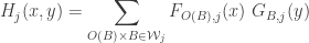
is well defined. Since \mathcal{B}_j is locally finite in Y, \mathcal{W}_j is locally finite in X \times Y. Thus H_j(x,y) is obtained by summing a finite number of values of F_{O(B),j}(x) \ G_{B,j}(y). On the other hand, it can be shown that H_j is continuous for each j. Based on the definition of H_j, it can be readily verified that H_j(x,y)>0 for all (x,y) \in \cup \mathcal{W}_j and H_j(x,y)=0 for all (x,y) \notin \cup \mathcal{W}_j.

Define H: X \times Y \rightarrow [0,1] by the following:

    \displaystyle H(x,y)=\sum \limits_{j=1}^\infty \biggl[ \frac{1}{2^j} \ \frac{H_j(x,y)}{1+H_j(x,y)} \biggr]

It is clear that H is continuous. We claim that U=\left\{(x,y) \in X \times Y: H(x,y) >0 \right\}. Recall that the open set U is the union of all O(B) \times B \in \mathcal{W}_j for all j. Thus if (x,y) \in \cup \mathcal{W}_j for some j, then H(x,y)>0 since H_j(x,y)>0. If (x,y) \notin \cup \mathcal{W}_j for all j, H(x,y)=0 since H_j(x,y)=0 for all j. Thus the open set U is an F_\sigma-subset of X \times Y. This concludes the proof that X \times Y is perfectly normal. \square

____________________________________________________________________

Remarks

The main theorem here is a classic result in general topology. An alternative proof is to show that any perfectly normal space is a P-space (definition given below). Then by Morita’s theorem, the product of any perfectly normal space and any metric space is normal (Theorem 1 below). For another proof that is elementary, see Lemma 7 in this previous post.

The notions of perfectly normal spaces and paracompact spaces are quite different. By the theorem discussed here, perfectly normal spaces are normally productive with metric spaces. It is possible for a paracompact space to have a non-normal product with a metric space. The classic example is the Michael line (discussed here).

On the other hand, there are perfectly normal spaces that are not paracompact. One example is Bing’s Example H, which is perfectly normal and not paracompact (see here).

Even though a perfectly normal space is normally productive with metric spaces, it cannot be normally productive in general. For each non-discrete perfectly normal space X, there exists a normal space Y such that X \times Y is not normal. This follows from Morita’s first conjecture (now a true statement). Morita’s first conjecture is discussed here.

____________________________________________________________________

P-Space in the Sense of Morita

Morita defined the notion of P-spaces [1] and [2]. Let \kappa be a cardinal number such that \kappa \ge 1. Let \Gamma be the set of all finite ordered sequences (\alpha_1,\alpha_2,\cdots,\alpha_n) where n=1,2,\cdots and all \alpha_i < \kappa. Let X be a space. The collection \left\{F_\sigma \subset X: \sigma \in \Gamma \right\} is said to be decreasing if this condition holds: \sigma =(\alpha_1,\alpha_2,\cdots,\alpha_n) and \delta =(\alpha_1,\alpha_2,\cdots,\alpha_n, \cdots, \alpha_m) with n<m imply that F_{\delta} \subset F_{\sigma}. The space X is a P-space if for any cardinal \kappa \ge 1 and for any decreasing collection \left\{F_\sigma \subset X: \sigma \in \Gamma \right\} of closed subsets of X, there exists open set U_\sigma for each \sigma \in \Gamma such that the following conditions hold:

  • for all \sigma \in \Gamma, F_\sigma \subset U_\sigma,
  • for any infinite sequence (\alpha_1,\alpha_2,\cdots,\alpha_n,\cdots) where each each finite subsequence \sigma_n=(\alpha_1,\alpha_2,\cdots,\alpha_n) is an element of \Gamma, if \bigcap_{n=1}^\infty F_{\sigma_n}=\varnothing, then \bigcap_{n=1}^\infty U_{\sigma_n}=\varnothing.

If \kappa=1 where 1=\left\{0 \right\}. Then the index set \Gamma defined above can be viewed as the set of all positive integers. As a result, the definition of P-space with \kappa=1 implies the a condition in Dowker’s theorem (see condition 6 in Theorem 1 here). Thus any space X that is normal and a P-space is countably paracompact (or countably shrinking or that X \times Y is normal for every compact metric space or any other equivalent condition in Dowker’s theorem). The following is a theorem of Morita.

Theorem 1 (Morita)
Let X be a space. Then X is a normal P-space if and only if X \times Y is normal for every metric space Y.

In light of Theorem 1, both perfectly normal spaces and normal countably compact spaces are P-spaces (see here). According to Theorem 1 and Dowker’s theorem, it follows that any normal P-space is countably paracompact.

____________________________________________________________________

Reference

  1. Morita K., On the Product of a Normal Space with a Metric Space, Proc. Japan Acad., Vol. 39, 148-150, 1963. (article information; paper)
  2. Morita K., Products of Normal Spaces with Metric Spaces, Math. Ann., Vol. 154, 365-382, 1964.

____________________________________________________________________
\copyright \ 2017 \text{ by Dan Ma}

The product of a normal countably compact space and a metric space is normal

It is well known that normality is not preserved by taking products. When nothing is known about the spaces X and Y other than the facts that they are normal spaces, there is not enough to go on for determining whether X \times Y is normal. In fact even when one factor is a metric space and the other factor is a hereditarily paracompact space, the product can be non-normal (discussed here). This post discusses a productive scenario – the first factor is a normal space and second factor is a metric space with the first factor having the additional property that it is countably compact. In this scenario the product is always normal. This is a well known result in general topology. The goal here is to nail down a proof for use as future reference.

Main Theorem
Let X be a normal and countably compact space. Then X \times Y is a normal space for every metric space Y.

The proof of the main theorem uses the notion of shrinkable open covers.

Remarks
The main theorem is a classic result and is often used as motivation for more advanced results for products of normal spaces. Thus we would like to present a clear and complete proof of this classic result for anyone who would like to study the topics of normality (or the lack of) in product spaces. We found that some proofs of this result in the literature are hard to follow. In A. H. Stone’s paper [2], the result is stated in a footnote, stating that “it can be shown that the topological product of a metric space and a normal countably compact space is normal, though not necessarily paracompact”. We had seen several other papers citing [2] as a reference for the result. The Handbook [1] also has a proof (Corollary 4.10 in page 805), which we feel may not be the best proof to learn from. We found a good proof in [3] using the idea of shrinking of open covers.

____________________________________________________________________

The Notion of Shrinking

The key to the proof is the notion of shrinkable open covers and shrinking spaces. Let X be a space. Let \mathcal{U} be an open cover of X. The open cover of \mathcal{U} is said to be shrinkable if there is an open cover \mathcal{V}=\left\{V(U): U \in \mathcal{U} \right\} of X such that \overline{V(U)} \subset U for each U \in \mathcal{U}. When this is the case, the open cover \mathcal{V} is said to be a shrinking of \mathcal{U}. If an open cover is shrinkable, we also say that the open cover can be shrunk (or has a shrinking). Whenever an open cover has a shrinking, the shrinking is indexed by the open cover that is being shrunk. Thus if the original cover is indexed, e.g. \left\{U_\alpha: \alpha<\kappa \right\}, then a shrinking has the same indexing, e.g. \left\{V_\alpha: \alpha<\kappa \right\}.

A space X is a shrinking space if every open cover of X is shrinkable. Every open cover of a paracompact space has a locally finite open refinement. With a little bit of rearranging, the locally finite open refinement can be made to be a shrinking (see Theorem 2 here). Thus every paracompact space is a shrinking space. For other spaces, the shrinking phenomenon is limited to certain types of open covers. In a normal space, every finite open cover has a shrinking, as stated in the following theorem.

Theorem 1
The following conditions are equivalent.

  1. The space X is normal.
  2. Every point-finite open cover of X is shrinkable.
  3. Every locally finite open cover of X is shrinkable.
  4. Every finite open cover of X is shrinkable.
  5. Every two-element open cover of X is shrinkable.

The hardest direction in the proof is 1 \Longrightarrow 2, which is established in this previous post. The directions 2 \Longrightarrow 3 \Longrightarrow 4 \Longrightarrow 5 are immediate. To see 5 \Longrightarrow 1, let H and K be two disjoint closed subsets of X. By condition 5, the two-element open cover \left\{X-H,X-K \right\} has a shrinking \left\{U,V \right\}. Then \overline{U} \subset X-H and \overline{V} \subset X-K. As a result, H \subset X-\overline{U} and K \subset X-\overline{V}. Since the open sets U and V cover the whole space, X-\overline{U} and X-\overline{V} are disjoint open sets. Thus X is normal.

In a normal space, all finite open covers are shrinkable. In general, an infinite open cover of a normal space may or may not be shrinkable. It turns out that finding a normal space with an infinite open cover that is not shrinkable is no trivial matter (see Dowker’s theorem in this previous post). However, if an open cover in a normal space is point-finite or locally finite, then it is shrinkable.

____________________________________________________________________

Key Idea

We now discuss the key idea to the proof of the main theorem. Consider the product space X \times Y. Let \mathcal{U} be an open cover of X \times Y. Let M \subset Y. The set M is stable with respect to the open cover \mathcal{U} if for each x \in X, there is an open set O_x containing x such that O_x \times M \subset U for some U \in \mathcal{U}.

Let \kappa be a cardinal number (either finite or infinite). A space X is a \kappa-shrinking space if for each open cover \mathcal{W} of X such that the cardinality of \mathcal{W} is \le \kappa, then \mathcal{W} is shrinkable. According to Theorem 1, any normal space is 2-shrinkable.

Theorem 2
Let \kappa be a cardinal number (either finite or infinite). Let X be a \kappa-shrinking space. Let Y be a paracompact space. Suppose that \mathcal{U} is an open cover of X \times Y such that the following two conditions are satisfied:

  • Each point y \in Y has an open set V_y containing y such that V_y is stable with respect to \mathcal{U}.
  • \lvert \mathcal{U} \lvert = \kappa.

Then \mathcal{U} is shrinkable.

Proof of Theorem 2
Let \mathcal{U} be any open cover of X \times Y satisfying the hypothesis. We show that \mathcal{U} has a shrinking.

For each y \in Y, obtain the open covers \left\{G(U,y): U \in \mathcal{U} \right\} and \left\{H(U,y): U \in \mathcal{U} \right\} of X as follows. For each U \in \mathcal{U}, define the following:

    G(U,y)=\cup \left\{O: O \text{ is open in } X \text{ such that } O \times V_y \subset U \right\}

Then \left\{G(U,y): U \in \mathcal{U} \right\} is an open cover of X. Since X is \kappa-shrinkable, there is an open cover \left\{H(U,y): U \in \mathcal{U} \right\} of X such that \overline{H(U,y)} \subset G(U,y) for each U \in \mathcal{U}.

Now \left\{V_y: y \in Y \right\} is an open cover of Y. By the paracompactness of Y, let \left\{W_y: y \in Y \right\} be a locally finite open cover of Y such that \overline{W_y} \subset V_y for each y \in Y. For each U \in \mathcal{U}, define the following:

    W_U=\cup \left\{H(U,y) \times W_y: y \in Y \text{ such that } \overline{H(U,y) \times W_y} \subset U \right\}

We claim that \mathcal{W}=\left\{ W_U: U \in \mathcal{U} \right\} is a shrinking of \mathcal{U}. First it is a cover of X \times Y. Let (x,t) \in X \times Y. Then t \in W_y for some y \in Y. There exists U \in \mathcal{U} such that x \in H(U,y). Note the following.

    \overline{H(U,y) \times W_y} \subset \overline{H(U,y)} \times \overline{W_y} \subset G(U,y) \times V_y \subset U

This means that H(U,y) \times W_y \subset W_U. Since (x,t) \in H(U,y) \times W_y, (x,t) \in W_U. Thus \mathcal{W} is an open cover of X \times Y.

Now we show that \mathcal{W} is a shrinking of \mathcal{U}. Let U \in \mathcal{U}. To show that \overline{W_U} \subset U, let (x,t) \in \overline{W_U}. Let L be open in Y such that t \in L and that L meets only finitely many W_y, say for y=y_1,y_2,\cdots,y_n. Immediately we have the following relations.

    \forall \ i=1,\cdots,n, \ \overline{W_{y_i}} \subset V_{y_i}

    \forall \ i=1,\cdots,n, \ \overline{H(U,y_i)} \subset G(U,y_i)

    \forall \ i=1,\cdots,n, \ \overline{H(U,y_i) \times W_{y_i}} \subset \overline{H(U,y_i)} \times \overline{W_{y_i}} \subset G(U,y_i) \times V_{y_i} \subset U

Then it follows that

    \displaystyle (x,t) \in \overline{\bigcup \limits_{j=1}^n H(U,y_j) \times W_{y_j}}=\bigcup \limits_{j=1}^n \overline{H(U,y_j) \times W_{y_j}} \subset U

Thus U \in \mathcal{U}. This shows that \mathcal{W} is a shrinking of \mathcal{U}. \square

Remark
Theorem 2 is the Theorem 3.2 in [3]. Theorem 2 is a formulation of Theorem 3.2 [3] for the purpose of proving Theorem 3 below.

____________________________________________________________________

Main Theorem

Theorem 3 (Main Theorem)
Let X be a normal and countably compact space. Let Y be a metric space. Then X \times Y is a normal space.

Proof of Theorem 3
Let \mathcal{U} be a 2-element open cover of X \times Y. We show that \mathcal{U} is shrinkable. This would mean that X \times Y is normal (according to Theorem 1). To show that \mathcal{U} is shrinkable, we show that the open cover \mathcal{U} satisfies the two bullet points in Theorem 2.

Fix y \in Y. Let \left\{B_n: n=1,2,3,\cdots \right\} be a base at the point y. Define G_n as follows:

    G_n=\cup \left\{O \subset X: O \text{ is open such that } O \times B_n \subset U \text{ for some } U \in \mathcal{U} \right\}

It is clear that \mathcal{G}=\left\{G_n: n=1,2,3,\cdots \right\} is an open cover of X. Since X is countably compact, choose m such that \left\{G_1,G_2,\cdots,G_m \right\} is a cover of X. Let E_y=\bigcap_{j=1}^m B_j. We claim that E_y is stable with respect to \mathcal{U}. To see this, let x \in X. Then x \in G_j for some j \le m. By the definition of G_j, there is some open set O_x \subset X such that x \in O_x and O_x \times B_j \subset U for some U \in \mathcal{U}. Furthermore, O_x \times E_y \subset O_x \times B_j \subset U.

To summarize: for each y \in Y, there is an open set E_y such that y \in E_y and E_y is stable with respect to the open cover \mathcal{U}. Thus the first bullet point of Theorem 2 is satisfied. The open cover \mathcal{U} is a 2-element open cover. Thus the second bullet point of Theorem 2 is satisfied. By Theorem 2, the open cover \mathcal{U} is shrinkable. Thus X \times Y is normal. \square

Corollary 4
Let X be a normal and pseudocompact space. Let Y be a metric space. Then X \times Y is a normal space.

The corollary follows from the fact that any normal and pseudocompact space is countably compact (see here).

Remarks
The proof of Theorem 3 actually gives a more general result. Note that the second factor only needs to be paracompact and that every point has a countable base (i.e. first countable). The first factor X has to be countably compact. The shrinking requirement for X is flexible – if open covers of a certain size for X are shrinkable, then open covers of that size for the product are shrinkable. We have the following corollaries.

Corollary 5
Let X be a \kappa-shrinking and countably compact space and let Y be a paracompact first countable space. Then X \times Y is a \kappa-shrinking space.

Corollary 6
Let X be a shrinking and countably compact space and let Y be a paracompact first countable space. Then X \times Y is a shrinking space.

____________________________________________________________________

Remarks

The main theorem (Theorem 3) says that any normal and countably compact space is productively normal with one class of spaces, namely the metric spaces. Thus if one wishes to find a non-normal product space with one factor being countably compact, the other factor must not be a metric space. For example, if W=\omega_1, the first uncountable ordinal with the ordered topology, then W \times X is always normal for every metric X. For non-normal example, W \times C is not normal for any compact space C with uncountable tightness (see Theorem 1 in this previous post). Another example, W \times L_{\omega_1} is not normal where L_{\omega_1} is the one-point Lindelofication of a discrete space of cardinality \omega_1 (follows from Example 1 and Theorem 7 in this previous post).

Another comment is that normal countably paracompact spaces are examples of Normal P-spaces. K. Morita defined the notion of P-space and he proved that a space Y is a Normal P-space if and only if X \times Y is normal for every metric space X.

____________________________________________________________________

Reference

  1. Przymusinski T. C., Products of Normal Spaces, Handbook of Set-Theoretic Topology (K. Kunen and J. E. Vaughan, eds), Elsevier Science Publishers B. V., Amsterdam, 781-826, 1984.
  2. Stone A. H., Paracompactness and Product Spaces, Bull. Amer. Math. Soc., Vol. 54, 977-982, 1948. (paper)
  3. Yang L., The Normality in Products with a Countably Compact Factor, Canad. Math. Bull., Vol. 41 (2), 245-251, 1998. (abstract, paper)

____________________________________________________________________
\copyright \ 2017 \text{ by Dan Ma}