Let  be a mapping from a topological space
  onto a topological space
  . If
. If  is a perfect map and is a Lindelof space, then so is . If is a closed map and is a paracompact space, then so is . In other words, the pre-image of a Lindelof space under a perfect map is always a Lindelof space. Likewise, the pre-image of a paracompact space under a closed map is always a paracompact space. After proving these two facts, we show that for any compact space , the product
  is Lindelof (paracompact) for any Lindelof (paracompact) space . All spaces under consideration are Hausdorff.
Another way to state the above two facts is that Lindelofness is an inverse invariance under perfect maps and that paracompactness is an inverse invariance of the closed maps. In general, a topological property is an inverse invariance of a class of mappings  if the following holds: for any mapping belonging to , if has the property, then so does . In contrast, a topological property is an invariance of a class of mappings if for any mapping belonging to , if has the property, then so does .
All mappings under consideration are continuous maps. A mapping , where  , is a closed map if for any closed subset
  of ,
of ,  is closed in . A mapping , where , is a perfect map if is a closed map and that the point inverse
  is compact for each
  .
.
Perfect mappings and closed mappings are objects with strong properties. Such a map places a restriction on what topological properties the “domain” space or the “range” space can have. The theorems below indicate that it is not possible to map a non-Lindelof space onto a Lindelof space using a perfect map and that it is not possible to map a non-paracompact space onto a paracompact space using a closed map. On the other hand, it is not possible to map a separable metric space onto a separable but non-metric space using a perfect map (see here). We prove the following theorems.
Theorem 1…. Lindelofness (or the Lindelof property) is an inverse invariant of the perfect maps.
Theorem 2 ….Paracompactness is an inverse invariant of the closed maps.
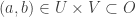
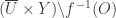
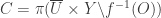
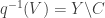
Lemma 3 …. Let  be a closed map with . Let
  be an open subset of . Define
  . Then the set
  is open in and that
  .
.
For the proof of Lemma 3, see Lemma 2 here.
Proof of Theorem 1
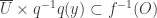
Let be a perfect map with . Suppose is Lindelof. Let  be an open cover of . Without loss of generality, we can assume that is closed under finite unions. For each
  , define
  . By Lemma 3, each
  is an open subset of . We claim that
  is an open cover of . To this end, let . Since is a perfect map, the point inverse is compact. As a result, we can find a finite
  such that
  . Since is closed under finite unions,
  . It follows that
  . Since is Lindelof, there exists a countable
  such that
  . For each
  ,
,  for some
  . We claim that
  is a cover of . To this end, let
  . Then for some ,
  . This implies that
  . Thus, the open cover has a countable subcover. This concludes the proof of Theorem 1.
Proof of Theorem 2
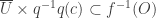
Let be a perfect map with . Suppose is paracompact. Let be an open cover of . For each , define as in Lemma 3. By Lemma 3, each is an open subset of . Let . As shown in the proof of Theorem 1,  is an open cover of . Since is paracompact, there exists a locally finite open refinement
  of . Let
  .
.
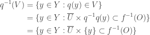
We show three facts about  . (1) It is an open cover of . (2) It is a locally finite collection in . (3) It is a refinement of . To see (1), note that is an open cover of . As a result, is an open cover of . To see (2), let . We find an open
  such that
  and such that
  intersects only finitely many elements of . Since is locally finite in , there exists an open
  such that
  and such that
  intersects only finitely many elements of , say,
  . Let
. Let  . Clearly, . It can be verified that the only elements of having non-empty intersections with are
  ,
, ,
, . To see (3), let
  where
where  . Then
  for some
  and some . We claim that
  . Let
. Let  . Then
  . This implies that
  . It follows that is a locally finite open refinement of the open cover . This completes the proof of Theorem 2.
Productively Paracompact Spaces
A space is productively paramcompact if is paracompact for every paracompact space . The definition for productively Lindelof can be stated in a similar way. For some reason, the term “productively paracompact” is not used in the literature but is a topic that had been extensively studied. It is also a topic found in this site. The following four classes of spaces are productively paracompact (see here and here).
- Compact spaces
 -compact spaces
- Locally compact spaces
- -locally compact spaces
The proof for compact spaces being productively paracompact given here uses the Tube Lemma (see here). As applications of Theorem 1 and Theorem 2, we use the two theorems to show that compact spaces are both productively Lindelof and productive paracompact.
Theorem 4…. Let any compact space. Then is Lindelof for every Lindelof space .
Theorem 5 ….Let any compact space. Then is paracompact for every paracompact space .
Theorems 4 and 5 are corollaries to the Kuratowski theorem (see here) and Theorems 1 and 2 above. Suppose is compact. Then the projection map from onto is a closed map. The paracompactness of follows whenever is paracompact. The projection map is also perfect since the point inverses are compact due to the compactness of the factor . Then the Lindelofness of follows whenever is Lindelof.

Dan Ma invariant
Daniel Ma invariant
Dan Ma Inverse invariant
Daniel Ma Inverse invariant
Dan Ma perfect map
Daniel Ma perfect map
Dan Ma paracompact space
Daniel Ma paracompact space
Dan Ma Lindelof space
Daniel Ma Lindelof space
Dan Ma topology
Daniel Ma topology
 2023 – Dan Ma


if and only if


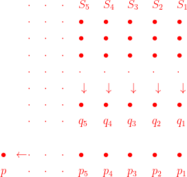
 going downward and going across from right to left. The point
  are situated below the points
  . In this Euclidean space, the points in the sequences
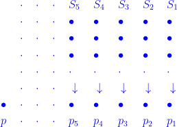
 be the set of all points
  with the quotient topology. With the quotient topology, an open set containing the point
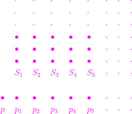
 consists of the point
  . Note that no sequence of points in
  . As observed in the preceding paragraph, no sequence of points in