Certain covering properties and separation properties allow open covers to shrink, e.g. paracompact spaces, normal spaces, and countably paracompact spaces. The shrinking property is also interesting on its own. This post gives a more in-depth discussion than the one in the previous post on countably paracompact spaces. After discussing shrinking spaces, we introduce three shrinking related properties. These properties show that there is a deep and delicate connection among shrinking properties and normality in products. This post is also a preparation for the next post on  -Dowker space and Morita’s first conjecture.
All spaces under consideration are Hausdorff and normal or Hausdorff and regular (if not normal).
____________________________________________________________________
Shrinking Spaces
Let  be a space. Let
  be an open cover of . The open cover of is said to be shrinkable if there is an open cover
  of such that
  for each
  . When this is the case, the open cover
  is said to be a shrinking of . If an open cover is shrinkable, we also say that the open cover can be shrunk (or has a shrinking). Whenever an open cover has a shrinking, the shrinking is indexed by the open cover that is being shrunk. Thus if the original cover is indexed in a certain way, e.g.
  , then a shrinking has the same indexing, e.g.
  .
.
A space is a shrinking space if every open cover of is shrinkable. The property can also be broken up according to the cardinality of the open cover. Let be a cardinal. A space is -shrinking if every open cover of cardinality  for is shrinkable. A space is countably shrinking if it is
  -shrinking.
____________________________________________________________________
Examples of Shrinking
Let’s look at a few situations where open covers can be shrunk either all the time or on a limited basis. For a normal space, certain covers can be shrunk as indicated by the following theorem.
Theorem 1
The following conditions are equivalent.
- The space is normal.
- Every point-finite open cover of is shrinkable.
- Every locally finite open cover of is shrinkable.
- Every finite open cover of is shrinkable.
- Every two-element open cover of is shrinkable.
The hardest direction in the proof is  , which is established in this previous post. The directions
  are immediate. To see
  , let
, let  and
and  be two disjoint closed subsets of . By condition 5, the two-element open cover
 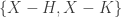 has a shrinking
  . Then
  and
and  . As a result,
  and
and  . Since the open sets
  and
and  cover the whole space,
  and
and  are disjoint open sets. Thus is normal.
In a normal space, all finite open covers are shrinkable. In general, an infinite open cover of a normal space does not have to be shrinkable unless it is a point-finite or locally finite open cover.
The theorem of C. H. Dowker states that a normal space is countably paracompact if and only every countable open cover of is shrinkable if and only if the product space  is normal for every compact metric space
  if and only if the product space
 ![X \times [0,1]](https://s0.wp.com/latex.php?latex=X+%5Ctimes+%5B0%2C1%5D&bg=ffffff&fg=333333&s=0&c=20201002) is normal. The theorem is discussed here. A Dowker space is a normal space that violates the theorem. Thus any Dowker space has a countably infinite open cover that cannot be shrunk, or equivalently a normal space that forms a non-normal product with a compact metric space. Thus the notion of shrinking has a connection with normality in the product spaces. A Dowker space space was constructed by M. E. Rudin in ZFC [2]. So far Rudin’s example is essentially the only ZFC Dowker space. This goes to show that finding a normal space that is not countably shrinking is not a trivial matter.
is normal. The theorem is discussed here. A Dowker space is a normal space that violates the theorem. Thus any Dowker space has a countably infinite open cover that cannot be shrunk, or equivalently a normal space that forms a non-normal product with a compact metric space. Thus the notion of shrinking has a connection with normality in the product spaces. A Dowker space space was constructed by M. E. Rudin in ZFC [2]. So far Rudin’s example is essentially the only ZFC Dowker space. This goes to show that finding a normal space that is not countably shrinking is not a trivial matter.
Several facts can be derived easily from Theorem 1 and Dowker’s theorem. For clarity, they are called out as corollaries.
Corollary 2
- All shrinking spaces are normal.
- All shrinking spaces are normal and countably paracompact.
- Any normal and metacompact space is a shrinking space.
For the first corollary, if every open cover of a space can be shrunk, then all finite open covers can be shrunk and thus the space must be normal. As indicated above, Dowker’s theorem states that in a normal space, countably paracompactness is equivalent to countably shrinking. Thus any shrinking space is normal and countably paracompact.
Though an infinite open cover of a normal space may not be shrinkable, adding an appropriate covering property to any normal space will make it into a shrinking space. An easy way is through point-finite open covers. If every open cover has a point-finite open refinement (i.e. a metacompact space), then the point-finite open refinement can be shrunk (if the space is also normal). Thus the third corollary is established. Note that the metacompact is not the best possible result. For example, it is known that any normal and submetacompact space is a shrinking space – see Theorem 6.2 of [1].
In paracompact spaces, all open covers can be shrunk. One way to see this is through Corollary 2. Any paracompact space is normal and metacompact. It is also informative to look at the following characterization of paracompact spaces.
Theorem 3
A space is paracompact if and only if every open cover of has a locally finite open refinement such that  for each
  .
.
A proof can be found here. Thus every open cover of a paracompact space can be shrunk by a locally finite shrinking. To summarize, we have discussed the following implications.
Diagram 1
____________________________________________________________________
Three Shrinking Related Properties
None of the implications in Diagram 1 can be reversed. The last implication in the diagram cannot be reversed due to Rudin’es Dowker space. One natural example to look for would be spaces that are normal and countably paracompact but fail in shrinking at some uncountable cardinal. As indicated by the the theorem of C. H, Dowker, the notion of shrinking is intimately connected to normality in product spaces . To further investigate, consider the following three properties.
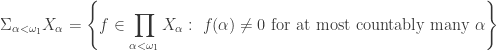
Let be a space. Let be an infinite cardinal. Consider the following three properties.
The space is -shrinking if and only if any open cover of cardinality for the space is shrinkable, i.e. the following condition holds.
For each open cover of , there exists an open cover such that for each  .
.
The space has Property  if and only if every increasing open cover of cardinality for the space is shrinkable, i.e. the following holds.
For each increasing open cover of , there exists an open cover such that for each .
The space has Property  if and only if the following holds.
For each increasing open cover of , there exists an increasing open cover such that for each .
A family  is increasing if
  for any
  . It is decreasing if
  for any .
In general, any space that is -shrinking for all cardinals is a shrinking space as defined earlier. Any space that has property for all cardinals is said to have property  . Any space that has property for all cardinals is said to have property
  .
.
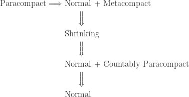
The first property -shrinking is simply the shrinking property for open covers of cardinality . The property is -shrinking with the additional requirement that the open covers to be shrunk must be increasing. It is clear that -shrinking implies property . The property appears to be similar to except that has the additional requirement that the shrinking is also increasing. As a result implies . The following diagram shows the implications.
Diagram 2
The implications in Diagram 2 are immediate. An example is given below showing that  -shrinking does not imply property
  . If
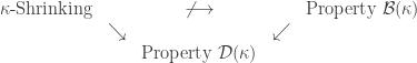
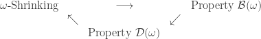
. If  , then all three properties are equivalent in normal spaces, as displayed in the following diagram. The proof is in Theorem 5.
Diagram 3
The property has a dual statement in terms of decreasing closed sets. The following theorem gives the dual statement.
Theorem 4
Let be a normal space. Let be an infinite cardinal. The following two properties are equivalent.
- The space has property .
- For each decreasing family
 of closed subsets of such that
  , there exists a family
  of open subsets of such that
  and
and  for each .
First bullet implies second bullet
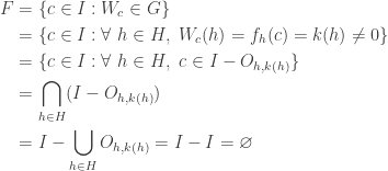
Let be a decreasing family of closed subsets of with empty intersection. Then is an increasing family of open subsets of where  . Let be an open cover of such that for each . Then where
  is the needed open expansion.
Second bullet implies first bullet
Let be an increasing open cover of . Then is a decreasing family of closed subsets of where  . Note that . Let be a family of open subsets of such that and for each . For each , there is open set
  such that
  since is normal. For each , let
  . Then is a family of open subsets of required by the first bullet. It is a cover because
  . To show , let
  such that
  . Then
  . Since and is open,
  . Let
. Let  . Since
  ,
,  , which means
  , a contradiction. Thus .
Now we show that the three properties in Diagram 3 are equivalent.
Theorem 5
Let be a normal space. Then the following implications hold.
-shrinking  Property
  Property
  -shrinking
Proof of Theorem 5
-shrinking Property
Suppose that is -shrinking. By Dowker’s theorem,  is a normal space. We can think of
  as a convergent sequence with as the limit point. Let
  be an increasing open cover of . Define and as follows:
It is straightforward to verify that and are disjoint closed subsets of . By normality, let and  be disjoint open subsets of such that
  and
and  . For each integer
  , define
  as follows:
The set ![[n, \omega]](https://s0.wp.com/latex.php?latex=%5Bn%2C+%5Comega%5D&bg=ffffff&fg=333333&s=0&c=20201002) consists of all integers
consists of all integers  and the limit point . From the way the sets are defined,
  is an increasing open cover of . The remaining thing to show is that
  for each
  . Suppose that
  and
and  . Then
  by definition of . There exists an open set
  such that
  and
and  . Since
  is an open set containing
  ,
,  . Let
. Let  . By definition of , there is some open set
  such that
  and
and ![O \times [n, \omega] \subset V](https://s0.wp.com/latex.php?latex=O+%5Ctimes+%5Bn%2C+%5Comega%5D+%5Csubset+V&bg=ffffff&fg=333333&s=0&c=20201002) , a contradiction since
, a contradiction since  is supposed to miss . Thus for all integers .
The direction Property Property is immediate.
Property -shrinking
Consider the dual condition of in Theorem 4, which is equivalent to -shrinking according to Dowker’s theorem. 
Remarks
The direction -shrinking Property is true because -shrinking is equivalent to the normality in the product . The same is not true when becomes an uncountable cardinal. We now show that -shrinking does not imply in general.
Example 1
The space  is the set of all ordinals less than with the ordered topology. Since it is a linearly ordered space, it is a shrinking space. Thus in particular it is -shrinking. To show that does not have property , consider the increasing open cover
  where
where  for each
  . Here
  consists of all ordinals less than . Suppose has property . Then let
  be an increasing open cover of such that for each .
Let  be the set of all limit ordinals in . For each
  ,
,  and thus
  . Thus there exists a countable ordinal
  such that
 ![(f(\alpha),\alpha]](https://s0.wp.com/latex.php?latex=%28f%28%5Calpha%29%2C%5Calpha%5D&bg=ffffff&fg=333333&s=0&c=20201002) misses points in
misses points in  . Thus the map
  is a pressing down map. By the pressing down lemma, there exists some such that
  is a stationary set in , which means that
  intersects with every closed and unbounded subset of . This means that for each
  ,
, ![(\alpha, \gamma]](https://s0.wp.com/latex.php?latex=%28%5Calpha%2C+%5Cgamma%5D&bg=ffffff&fg=333333&s=0&c=20201002) would miss
would miss  . This means that for each ,
 ![\overline{V_\gamma} \subset [0,\alpha]](https://s0.wp.com/latex.php?latex=%5Coverline%7BV_%5Cgamma%7D+%5Csubset+%5B0%2C%5Calpha%5D&bg=ffffff&fg=333333&s=0&c=20201002) . As a result would not be a cover of , a contradiction. So does not have property .
. As a result would not be a cover of , a contradiction. So does not have property .
____________________________________________________________________
Property
Of the three properties discussed in the above section, we would like to single out property . This property has a connection with normality in the product (see Theorem 7). First, we prove a lemma that is used in proving Theorem 7.
Lemma 6
Show that the property is hereditary with respect to closed subsets.
Proof of Lemma 6
Let be a space with property . Let  be a closed subspace of . Let
  be an increasing open cover of . For each , let be an open subset of such that
  . Since the open sets
  are increasing, the open sets can be chosen inductively such that
  for all
  . This will ensure that will form an increasing cover.
Then  is an increasing open cover of where
  . By property , let
  be an increasing open cover of such that
  . For each , let
  . It can be readily verified that
  is an increasing open cover of . Furthermore, for each (closure taken in ).
Let be an infinite cardinal. Let  be a discrete space of cardinality . Let
  be a point not in
  . Let
. Let  . Define a topology on
  by letting be discrete and by letting open neighborhood of be of the form
  where
where  and
and  has cardinality less than . Note the similarity between and the convergent sequence in the proof of Theorem 5.
Theorem 7
Let be a normal space. Then the product space  is normal if and only if has property .
Remarks
The property involves the shrinking of any increasing open cover with the added property that the shrinking is also increasing. The increasing shrinking is just what is needed to show that disjoint closed subsets of the product space can be separated.
Notations
Let’s set some notations that are useful in proving Theorem 7.
- The set
![[d_\alpha,p]](https://s0.wp.com/latex.php?latex=%5Bd_%5Calpha%2Cp%5D&bg=ffffff&fg=333333&s=0&c=20201002) is an open set in containing the point and is defined as follows.
is an open set in containing the point and is defined as follows.
![[d_\alpha,p]=\left\{d_\beta: \alpha \le \beta<\kappa \right\} \cup \left\{p \right\}](https://s0.wp.com/latex.php?latex=%5Bd_%5Calpha%2Cp%5D%3D%5Cleft%5C%7Bd_%5Cbeta%3A+%5Calpha+%5Cle+%5Cbeta%3C%5Ckappa+%5Cright%5C%7D+%5Ccup+%5Cleft%5C%7Bp+%5Cright%5C%7D&bg=ffffff&fg=333333&s=0&c=20201002) .
.
- For any two disjoint closed subsets and of the product space , define the following sets.
- For each , let
 and
and  .
.
- Let
 and
and  .
.
- For each , choose open
 such that
  ,
,  and
and  (due to normality of ).
- Choose open
 such that
  ,
,  and
and  (due to normality of ).
Proof of Theorem 7
Suppose that has property . Let and be two disjoint closed sets of . Consider the following cases based on the locations of the closed sets and .
Case 1.  and
and  .
.
Case 2a. 
Case 2b. Exactly one of and intersect the set  .
.
Case 3. Both and intersect the set .
Remarks
Case 1 is easy. Case 2a is the pivotal case. Case 2b and Case 3 use a similar idea. The result in Theorem 7 is found in [1] (Theorem 6.9 in p. 189) and [4]. The authors in these two sources claimed that Case 2a is the only case that matters, citing a lemma in another source. The lemma was not stated in these two sources and the source for the lemma is a PhD dissertation that is not readily available. Case 3 essentially uses the same idea but it has enough differences. For the sake of completeness, we work out all the cases. Case 3 applies property twice. Despite the complicated notations, the essential idea is quite simple. If any reader finds the proof too long, just understand Case 2a and then get the gist of how the idea is applied in Case 2b and Case 3.
Case 1.
and .
Let  . It is clear that
  and
and  .
.
Case 2a.
Assume that . We now proceed to separate and with disjoint open sets. For each , define as follows:
Then is an increasing open cover of . By property , there is an increasing open cover  of such that for each . The shrinking allows us to define an open set
  such that
  and
and  .
.
Let ![G=\cup \left\{V_\alpha \times [d_\alpha,p]: \alpha<\kappa \right\}](https://s0.wp.com/latex.php?latex=G%3D%5Ccup+%5Cleft%5C%7BV_%5Calpha+%5Ctimes+%5Bd_%5Calpha%2Cp%5D%3A+%5Calpha%3C%5Ckappa+%5Cright%5C%7D&bg=ffffff&fg=333333&s=0&c=20201002) . It is clear that . Next, we show that . Suppose that
. It is clear that . Next, we show that . Suppose that  . Then
 ![(x,d_\alpha) \notin U_\alpha \times [d_\alpha,p]](https://s0.wp.com/latex.php?latex=%28x%2Cd_%5Calpha%29+%5Cnotin+U_%5Calpha+%5Ctimes+%5Bd_%5Calpha%2Cp%5D&bg=ffffff&fg=333333&s=0&c=20201002) . As a result,
. As a result, ![(x,d_\alpha) \notin \overline{V_\alpha} \times [d_\alpha,p]](https://s0.wp.com/latex.php?latex=%28x%2Cd_%5Calpha%29+%5Cnotin+%5Coverline%7BV_%5Calpha%7D+%5Ctimes+%5Bd_%5Calpha%2Cp%5D&bg=ffffff&fg=333333&s=0&c=20201002) . Let
. Let  be open such that
  and
and ![(O \times \left\{d_\alpha \right\}) \cap (\overline{V_\alpha} \times [d_\alpha,p])=\varnothing](https://s0.wp.com/latex.php?latex=%28O+%5Ctimes+%5Cleft%5C%7Bd_%5Calpha+%5Cright%5C%7D%29+%5Ccap+%28%5Coverline%7BV_%5Calpha%7D+%5Ctimes+%5Bd_%5Calpha%2Cp%5D%29%3D%5Cvarnothing&bg=ffffff&fg=333333&s=0&c=20201002) . Since
. Since  for all
  , it follows that
 ![(O \times \left\{d_\alpha \right\}) \cap (V_\beta \times [d_\beta,p])=\varnothing](https://s0.wp.com/latex.php?latex=%28O+%5Ctimes+%5Cleft%5C%7Bd_%5Calpha+%5Cright%5C%7D%29+%5Ccap+%28V_%5Cbeta+%5Ctimes+%5Bd_%5Cbeta%2Cp%5D%29%3D%5Cvarnothing&bg=ffffff&fg=333333&s=0&c=20201002) for all
for all  . It is clear that
 ![(O \times \left\{d_\alpha \right\}) \cap (V_\gamma \times [d_\gamma,p])=\varnothing](https://s0.wp.com/latex.php?latex=%28O+%5Ctimes+%5Cleft%5C%7Bd_%5Calpha+%5Cright%5C%7D%29+%5Ccap+%28V_%5Cgamma+%5Ctimes+%5Bd_%5Cgamma%2Cp%5D%29%3D%5Cvarnothing&bg=ffffff&fg=333333&s=0&c=20201002) for all . What has been shown is that there is an open set containing the point
for all . What has been shown is that there is an open set containing the point  that contains no point of . This means that
  . We have established that .
Case 2b.
Exactly one of and intersect the set . We assume that is the set that intersects the set . The only difference between Case 2b and Case 2a is that there can be points of outside of in Case 2b.
Now proceed as in Case 2a. Obtain the open cover , the open cover and the open set as in Case 2a. Let  . It is clear that . We claim that . Suppose that
  . Since (as in Case 2a), there exists open set
  such that
  and
and  . There also exists open
  such that
  and
and  . It is clear that
  for all
  . This means that
  is an open set containing the point
  such that misses the open set
  . Thus .
Case 3.
Both and intersect the set .
Now project  and
and  onto the space .
Note that  is simply the copy of and
  is the copy of in . Since is normal, choose disjoint open sets
  and such that
  and
and  .
.
Let  and
and  . Let
. Let  and
and  . Note that
  is closed in ,
  is open in and
  . Similarly
  is closed in ,
  is open in and
  .
.
We now define two increasing open covers using property . Define  and
and  and
and  and
and  as follows:
The open cover  is an increasing open cover of . The open cover
  is an increasing open cover of .By property of and , both covers have the following as shrinking (by Lemma 6). The two shrinkings are:
such that
for each and such that both  and
and  are increasing open covers. Note that the closure
  is taken in and the closure
  is taken in .
For each , let  be the interior of
  and
and  be the interior of
  (with respect to ). Note that is meaningful since is a subset of the closure of the open set . Similar observation for . To make the rest of the argument easier to see, note the following fact about and .
For each , choose open set such that
The last point is possible because ![U_{\alpha,2} \times [d_\alpha,p]](https://s0.wp.com/latex.php?latex=U_%7B%5Calpha%2C2%7D+%5Ctimes+%5Bd_%5Calpha%2Cp%5D&bg=ffffff&fg=333333&s=0&c=20201002) misses and
misses and  . Define the open sets and as follows:
It is clear that . We claim that . To this end, we show that if  , then
  . If , then either
  for some
  or
or  .
.
Let . Note that ![(x,d_\gamma) \notin U_{\gamma,1} \times [d_\gamma,p]](https://s0.wp.com/latex.php?latex=%28x%2Cd_%5Cgamma%29+%5Cnotin+U_%7B%5Cgamma%2C1%7D+%5Ctimes+%5Bd_%5Cgamma%2Cp%5D&bg=ffffff&fg=333333&s=0&c=20201002) . Since
. Since  ,
, ![(x,d_\gamma) \notin \overline{W_{\gamma,1}} \times [d_\gamma,p]](https://s0.wp.com/latex.php?latex=%28x%2Cd_%5Cgamma%29+%5Cnotin+%5Coverline%7BW_%7B%5Cgamma%2C1%7D%7D+%5Ctimes+%5Bd_%5Cgamma%2Cp%5D&bg=ffffff&fg=333333&s=0&c=20201002) . Choose an open set such that and
. Choose an open set such that and  misses
 ![\overline{W_{\gamma,1}} \times [d_\gamma,p]](https://s0.wp.com/latex.php?latex=%5Coverline%7BW_%7B%5Cgamma%2C1%7D%7D+%5Ctimes+%5Bd_%5Cgamma%2Cp%5D&bg=ffffff&fg=333333&s=0&c=20201002) . Note that
. Note that  misses
 ![W_{\beta,1} \times [d_\beta,p]](https://s0.wp.com/latex.php?latex=W_%7B%5Cbeta%2C1%7D+%5Ctimes+%5Bd_%5Cbeta%2Cp%5D&bg=ffffff&fg=333333&s=0&c=20201002) for all
for all  since
since  for all . It is clear that misses for all
  .
.
We can also choose open  such that
  and
and  misses
  . It is clear that misses
  for all . Thus there is an open set containing the point such that contains no point of .
Let  . First we find an open set
  containing
  such that misses . From the way the open sets are defined, it follows that
 ![(x,p) \notin \overline{W_{\alpha,1}} \times [d_\alpha,p]](https://s0.wp.com/latex.php?latex=%28x%2Cp%29+%5Cnotin+%5Coverline%7BW_%7B%5Calpha%2C1%7D%7D+%5Ctimes+%5Bd_%5Calpha%2Cp%5D&bg=ffffff&fg=333333&s=0&c=20201002) for all . Furthermore
for all . Furthermore  . Thus
  is the desired open set. On the other hand, there exists such that
  . Note that
  are chosen so that
 ![(W_{\gamma,2} \times [d_\gamma,p]) \cap L_\gamma=\varnothing](https://s0.wp.com/latex.php?latex=%28W_%7B%5Cgamma%2C2%7D+%5Ctimes+%5Bd_%5Cgamma%2Cp%5D%29+%5Ccap+L_%5Cgamma%3D%5Cvarnothing&bg=ffffff&fg=333333&s=0&c=20201002) for all . Since
for all . Since  for all
  ,
, ![(W_{\alpha,2} \times [d_\alpha,p]) \cap L_\beta=\varnothing](https://s0.wp.com/latex.php?latex=%28W_%7B%5Calpha%2C2%7D+%5Ctimes+%5Bd_%5Calpha%2Cp%5D%29+%5Ccap+L_%5Cbeta%3D%5Cvarnothing&bg=ffffff&fg=333333&s=0&c=20201002) for all . Thus the open set
for all . Thus the open set ![W_{\alpha,2} \times [d_\alpha,p]](https://s0.wp.com/latex.php?latex=W_%7B%5Calpha%2C2%7D+%5Ctimes+%5Bd_%5Calpha%2Cp%5D&bg=ffffff&fg=333333&s=0&c=20201002) contains no points of for any . Then the open set
contains no points of for any . Then the open set ![Q \cap (W_{\alpha,2} \times [d_\alpha,p])](https://s0.wp.com/latex.php?latex=Q+%5Ccap+%28W_%7B%5Calpha%2C2%7D+%5Ctimes+%5Bd_%5Calpha%2Cp%5D%29&bg=ffffff&fg=333333&s=0&c=20201002) contains no point of . This means that
contains no point of . This means that  . Thus .
In each of the four cases (1, 2a, 2b and 3), there exists an open set  such that and . This completes the proof that is normal assuming that has property .
Now the other direction. Suppose that is normal. Then it can be shown that has property . The proof is similar to the proof for -shrinking Property in Theorem 5.
____________________________________________________________________
Reference
- Morita K., Nagata J.,Topics in General Topology, Elsevier Science Publishers, B. V., The Netherlands, 1989.
- Rudin M. E., A Normal Space for which
 is not Normal, Fund. Math., 73, 179-486, 1971. (link)
- Rudin M. E., Dowker Spaces, Handbook of Set-Theoretic Topology (K. Kunen and J. E. Vaughan, eds), Elsevier Science Publishers B. V., Amsterdam, (1984) 761-780.
- Yasui Y., On the Characterization of the -Property by the Normality of Product Spaces, Topology and its Applications, 15, 323-326, 1983. (abstract and paper)
- Yasui Y., Some Characterization of a -Property, TSUKUBA J. MATH., 10, No. 2, 243-247, 1986.
____________________________________________________________________


![I=[0,1]](https://s0.wp.com/latex.php?latex=I%3D%5B0%2C1%5D&bg=ffffff&fg=333333&s=0&c=20201002)


![\omega_1+1=[0, \omega_1]](https://s0.wp.com/latex.php?latex=%5Comega_1%2B1%3D%5B0%2C+%5Comega_1%5D&bg=ffffff&fg=333333&s=0&c=20201002)
![[0, \omega_1) \times [0, \omega_1]](https://s0.wp.com/latex.php?latex=%5B0%2C+%5Comega_1%29+%5Ctimes+%5B0%2C+%5Comega_1%5D&bg=ffffff&fg=333333&s=0&c=20201002)
![[0, \omega_1]](https://s0.wp.com/latex.php?latex=%5B0%2C+%5Comega_1%5D&bg=ffffff&fg=333333&s=0&c=20201002)


![[0,\omega_1]](https://s0.wp.com/latex.php?latex=%5B0%2C%5Comega_1%5D&bg=ffffff&fg=333333&s=0&c=20201002)
is normal.


 -compact spaces is a Lindelof space. The result is an example of a situation where the Lindelof property is countably productive if each factor is a “nice” Lindelof space. In this case, “nice” means
 ![\mathbb{R}=\bigcup_{n=1}^\infty [-n,n]](https://s0.wp.com/latex.php?latex=%5Cmathbb%7BR%7D%3D%5Cbigcup_%7Bn%3D1%7D%5E%5Cinfty+%5B-n%2Cn%5D&bg=ffffff&fg=333333&s=0&c=20201002) , the real line with the usual Euclidean topology is
, the real line with the usual Euclidean topology is  , the product of countably many copies of the real line, is not
  has a closed and discrete subspace of cardinality continuum where
  is cardinality of continuum. Hence
  has a closed and discrete subspace of cardinality
  be the set of all irrational numbers. Show that
  . The real line with this topology is called the Sorgenfrey line. Show that
  where
where  . Then there exists an open subset
 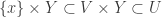 .
. is homeomorphic to the open interval
  ,
,  . Show that
  , the set of all non-negative integers. Since
  is a closed subset of
  , any closed and discrete subset of
  . To this end, we define
  after setting up background information.
 , choose a sequence
 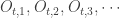 of open intervals (in the usual topology of
 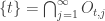 ,
, for each
  (the closure is in the usual topology of
  , the open intervals
  are of the form
  . For
. For  , the open intervals
  . For
. For  , the open intervals
 ![(a,1]](https://s0.wp.com/latex.php?latex=%28a%2C1%5D&bg=ffffff&fg=333333&s=0&c=20201002) .
.  as follows:
 ,
,  is the mapping
  defined by
  for each
  . If we replace open sets by open intervals, we have the same notion.
 is not Lindelof.
![[0,1]^\omega](https://s0.wp.com/latex.php?latex=%5B0%2C1%5D%5E%5Comega&bg=ffffff&fg=333333&s=0&c=20201002) . Since
. Since  of open and dense subsets of
  is a dense subset of
  be a sequence of non-empty open subsets of
  for each
  is non-empty.
 -subset of
  is a dense subset of
 ![X=[0,1]^\omega](https://s0.wp.com/latex.php?latex=X%3D%5B0%2C1%5D%5E%5Comega&bg=ffffff&fg=333333&s=0&c=20201002) is compact, it follows from Fact E.2 that the product space
is compact, it follows from Fact E.2 that the product space  . The product space
  for
for  . This follows from the definition of the mapping
  . Note that
  . Further note that
  for all
  .
. such that
  . Consider two cases.
 for all
  .
. is an open cover of
  such that
  is a cover of
  . Define the set
  as follows:
 because
  means that
  such that
  for some
  for all
  . This means that
  for some
 . Observe that
  since
since  . For each
  ,
,  since
since  . Thus
  .
. where each
  is a compact space as a subspace of
  where
where  is any rational number is also a closed and nowhere dense subset of
  be finite such that
  is a cover of
  . Putting it another way,
  . By the Tube lemma, for each
  such that
  . Since
  such that
  is a cover of
  is a countable subcover of
  . Choose
  . There must exist some
  such that
  . Choose
  . There must exist some
  such that
  . Continue in this manner we can choose inductively an infinite set
  such that
  for
for  . Since
  (in fact for infinitely many
  . Thus
  . We can choose an open set
  and
and  . However,
  . This is a contradiction since
  for all
  be open subsets of
  is also a dense subset of
  is dense in
  is non-empty. Since
  is dense in
  such that
  and
and  . Since
  is dense in
  such that
  and
and  . Continue inductively in this manner and we have a sequence of open sets
  is non-empty. Points in the intersection are in
  . This completes the proof of Fact E.2.
 where each
  is compact. Each
  . Since
  , there exists a non-empty open
  such that
  . This shows that each
  where each
  is a closed nowhere dense subset of
 and
and  are open and dense subsets of
  where for each integer
![U_n=(0,1) \times \cdots \times (0,1) \times [0,1] \times [0,1] \times \cdots](https://s0.wp.com/latex.php?latex=U_n%3D%280%2C1%29+%5Ctimes+%5Ccdots+%5Ctimes+%280%2C1%29+%5Ctimes+%5B0%2C1%5D+%5Ctimes+%5B0%2C1%5D+%5Ctimes+%5Ccdots&bg=ffffff&fg=333333&s=0&c=20201002)
![[0,1]](https://s0.wp.com/latex.php?latex=%5B0%2C1%5D&bg=ffffff&fg=333333&s=0&c=20201002) . It is also clear that
. It is also clear that  has uncountable extent where
  as a closed subspace. The non-normality of
  , the set of all rational numbers (a countable set). In this case,
  , the complement of a set
  , the product of countably many copies of the real line. The hints given use a Baire category argument, as outlined in Fact E.1 through Fact E.4. The product space
 ![[0,1]^{\omega}](https://s0.wp.com/latex.php?latex=%5B0%2C1%5D%5E%7B%5Comega%7D&bg=ffffff&fg=333333&s=0&c=20201002) , which is a Baire space. As mentioned earlier, Fact E.3 is essentially the same argument used for Exercise 2.B.
, which is a Baire space. As mentioned earlier, Fact E.3 is essentially the same argument used for Exercise 2.B. , the product of countably many copies of the countably infinite discrete space, is not
  be
be  is Lindelof.
 , let
, let  be compact spaces and let
  be the topological sum:
 is Lindelof.
 , the spaces
  are considered pairwise disjoint. The open sets in the sum are simply unions of the open sets in the individual spaces. Another way to view this topology: each of the
  is both closed and open in the topological sum. Theorem 2 is essentially saying that the product of countably many
  be a compact space. Let
  , closed subsets of
  where
where  , there exists
  such that
  and
and  . Then
  be the one-point compactification of
  is a compact space. Furthermore,
  is a subspace of
  , choose
  . Make sure that
  for
for 
 is of the form
  where
where  is open in
  . If
. If  , then
  .
.  . Let
. Let  , which is compact. We make the following claim.
 where
where  is finite and
  . Then
  .
. , there exists
  such that
  and
and  . This means that
  is an open cover of
  such that
  misses
  . Note that
  . Further note that
  . This establishes the claim that
  . The claim that
  is clear from the definition of
  such that
  , define
  . For integers
  , define the product
  as follows:
 and
and  . There exists an integer
  . This means that
  for all
  (so
(so  must be the point at infinity). Choose
  large enough such that
 . It follows that
  and
and  . Thus the sequence of closed sets
  , there is an open subset
  and
and  is compact. When we say
  where each
  is a locally compact space. In proving the result discussed here, we also assume that each
  of
of  is a locally finite family consisting of compact sets.
 such that each
  is closed and is locally compact. Fix an integer
  , let
, let  be an open subset of
  and
and  is compact (the closure is taken in
  of
of  be a locally finite open cover of
  for each
  is compact since
  . Let
. Let  .
. is a locally finite family with respect to the space
  ,
,  is an open set containing
  that meets only finitely many sets in
  of
of  . It is clear that
  be a
be a  and for each
  is obviously compact.
  , the point
  for some
  . Choose open
  and open
  such that
  . Letting
  cover the compact set
  be the intersection of these finitely many
  . Let
. Let  be the set of these finitely many
  .
. ,
, ,
,  for some
  such that
  for all

 is a
is a  . Then for some
  for some
  . Furthermore,
  for some
  . We now have
  .
. . Immediately we see that
  .
. is a locally finite family of open subsets of
  such that
  and
and  . Recall that
  is the set of all
  and is locally finite. Thus there exists an open
  and
and  . Thus the open set
  for finitely many
  meets only finitely many sets
  in
in 
 be the Michael line. Let
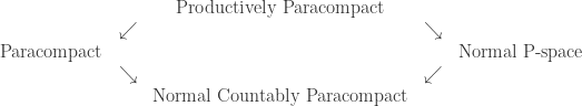
 -subset of the space
  is an
is an ![f: X \rightarrow [0,1]](https://s0.wp.com/latex.php?latex=f%3A+X+%5Crightarrow+%5B0%2C1%5D&bg=ffffff&fg=333333&s=0&c=20201002) such that
such that  , where
  . A subset
  is a zero-set, or more explicitly if there is a continuous function
  .
. be a base for
  is locally finite. We show that
  , there exists open
  and there exists
  such that
  . Then
  . Observe that
  for some integer
  such that
  for some
  be the union of all corresponding open sets
  for all applicable
  .
. be the collection of all open sets
  such that
  and
and  . As a result,
  .
. , there exist continuous functions
![F_{O(B),j}: X \rightarrow [0,1]](https://s0.wp.com/latex.php?latex=F_%7BO%28B%29%2Cj%7D%3A+X+%5Crightarrow+%5B0%2C1%5D&bg=ffffff&fg=333333&s=0&c=20201002)
![G_{B,j}: Y \rightarrow [0,1]](https://s0.wp.com/latex.php?latex=G_%7BB%2Cj%7D%3A+Y+%5Crightarrow+%5B0%2C1%5D&bg=ffffff&fg=333333&s=0&c=20201002)


![H_j: X \times Y \rightarrow [0,1]](https://s0.wp.com/latex.php?latex=H_j%3A+X+%5Ctimes+Y+%5Crightarrow+%5B0%2C1%5D&bg=ffffff&fg=333333&s=0&c=20201002) by the following:
by the following: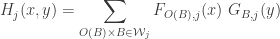
 is well defined. Since
  is obtained by summing a finite number of values of
  . On the other hand, it can be shown that
  for all
  and
and  for all
  .
.![H: X \times Y \rightarrow [0,1]](https://s0.wp.com/latex.php?latex=H%3A+X+%5Ctimes+Y+%5Crightarrow+%5B0%2C1%5D&bg=ffffff&fg=333333&s=0&c=20201002) by the following:
by the following:![\displaystyle H(x,y)=\sum \limits_{j=1}^\infty \biggl[ \frac{1}{2^j} \ \frac{H_j(x,y)}{1+H_j(x,y)} \biggr]](https://s0.wp.com/latex.php?latex=%5Cdisplaystyle+H%28x%2Cy%29%3D%5Csum+%5Climits_%7Bj%3D1%7D%5E%5Cinfty+%5Cbiggl%5B+%5Cfrac%7B1%7D%7B2%5Ej%7D+%5C+%5Cfrac%7BH_j%28x%2Cy%29%7D%7B1%2BH_j%28x%2Cy%29%7D+%5Cbiggr%5D&bg=ffffff&fg=333333&s=0&c=20201002)
 . Recall that the open set
  since
since  since
since  . Let
. Let  be the set of all finite ordered sequences
  where
where  and all
  . Let
. Let  is said to be decreasing if this condition holds:
  and
and  with
with  imply that
  . The space
  for each
  such that the following conditions hold:
 ,
, where each each finite subsequence
  is an element of
  , then
  .
. where
where  . Then the index set
  . The set
  for some
  of
of  has an open set
  containing
  .
. and
and  of
of 
 for each
  is an open cover of
  be a locally finite open cover of
  for each
 is a shrinking of
  . Then
  for some
  . Note the following.
 . Since
  ,
,  . Thus
  , let
, let  . Let
. Let  and that
  , say for
  . Immediately we have the following relations.


 be a base at the point
  as follows:
 is an open cover of
  such that
  is a cover of
  . We claim that
  is stable with respect to
  for some
  . By the definition of
  , there is some open set
  such that
  and
and  for some
  .
. and
and  , the first uncountable ordinal with the ordered topology, then
  is always normal for every metric
  is not normal for any compact space
  is not normal where
  is the one-point Lindelofication of a discrete space of cardinality
  is an open cover of
  such that
  of closed subsets of
  and
and  , there exist open sets
  such that
  for each
  .
. (as a subspace of the real line). Thus Rudin’s Dowker space has non-normal product with
  of subsets of the space
  whenever
  has a locally finite open refinement. Thus a space is paracompact if it is
  where
where  and
and  . In other words, any open set containing
  as the least infinite cardinal
  . For any non-discrete space
  for some infinite
  . For any space
  if and only if
 and
and  .
. and
and  are immediate. The following implications are established in
  (Theorem 4)
 (Theorem 7)
 and
and  .
. be an increasing open cover of
  be a locally finite open refinement of
 is still a locally finite refinement of
  be a shrinking of
  . Then
 for all
  . Suppose that
  be a non-discrete subset of
  for all
  ). Let
  be a decreasing family of closed subsets of

 . Two cases to consider:
  or
or  where
where  is the first closed set in the family
  .
. be least such that
  . Then
  for all
  since
since  is a closed set. Let
  , which is open containing
  . Then
  and
and  misses points of
  is an open set containing
  such that
  and
and  . For each
  as follows:
 . Choose an open set
  such that
  and
and  . Since
  , there is some
  such that
  . Since
  ,
,  . Thus
  . This establishes the claim that
  .
.
 and
and  . What about
  ? In [5], Beslagic and Rudin showed that
  using
using  . A natural question would be: can there be ZFC example? Perhaps searching on more recent papers can yield some answers.
 and
and  ? We do not know the answer.
 is not normal. Here
  is simply the one-point Lindelofication of a discrete space of cardinality

![V_n=\left\{x \in X: \exists \ \text{open } O \subset X \text{ such that } x \in O \text{ and } O \times [n, \omega] \subset V \right\}](https://s0.wp.com/latex.php?latex=V_n%3D%5Cleft%5C%7Bx+%5Cin+X%3A+%5Cexists+%5C+%5Ctext%7Bopen+%7D+O+%5Csubset+X+%5Ctext%7B+such+that+%7D+x+%5Cin+O+%5Ctext%7B+and+%7D+O+%5Ctimes+%5Bn%2C+%5Comega%5D+%5Csubset+V+%5Cright%5C%7D&bg=ffffff&fg=333333&s=0&c=20201002)
![U_\alpha=\cup \left\{O \subset X: O \text{ is open such that } (O \times [d_\alpha,p]) \cap K =\varnothing \right\}](https://s0.wp.com/latex.php?latex=U_%5Calpha%3D%5Ccup+%5Cleft%5C%7BO+%5Csubset+X%3A+O+%5Ctext%7B+is+open+such+that+%7D+%28O+%5Ctimes+%5Bd_%5Calpha%2Cp%5D%29+%5Ccap+K+%3D%5Cvarnothing+%5Cright%5C%7D&bg=ffffff&fg=333333&s=0&c=20201002)
![U_{\alpha,1}=\cup \left\{O \subset B_1: O \text{ is open such that } (O \times [d_\alpha,p]) \cap K =\varnothing \right\}](https://s0.wp.com/latex.php?latex=U_%7B%5Calpha%2C1%7D%3D%5Ccup+%5Cleft%5C%7BO+%5Csubset+B_1%3A+O+%5Ctext%7B+is+open+such+that+%7D+%28O+%5Ctimes+%5Bd_%5Calpha%2Cp%5D%29+%5Ccap+K+%3D%5Cvarnothing+%5Cright%5C%7D&bg=ffffff&fg=333333&s=0&c=20201002)
![U_{\alpha,2}=\cup \left\{O \subset B_2: O \text{ is open such that } (O \times [d_\alpha,p]) \cap H =\varnothing \right\}](https://s0.wp.com/latex.php?latex=U_%7B%5Calpha%2C2%7D%3D%5Ccup+%5Cleft%5C%7BO+%5Csubset+B_2%3A+O+%5Ctext%7B+is+open+such+that+%7D+%28O+%5Ctimes+%5Bd_%5Calpha%2Cp%5D%29+%5Ccap+H+%3D%5Cvarnothing+%5Cright%5C%7D&bg=ffffff&fg=333333&s=0&c=20201002)


 (closure with respect to
  (closure with respect to


![L_\alpha \cap (\overline{W_{\alpha,2}} \times [d_\alpha,p])=\varnothing](https://s0.wp.com/latex.php?latex=L_%5Calpha+%5Ccap+%28%5Coverline%7BW_%7B%5Calpha%2C2%7D%7D+%5Ctimes+%5Bd_%5Calpha%2Cp%5D%29%3D%5Cvarnothing&bg=ffffff&fg=333333&s=0&c=20201002)
![G=\cup \left\{W_{\alpha,1} \times [d_\alpha,p]: \alpha<\kappa \right\}](https://s0.wp.com/latex.php?latex=G%3D%5Ccup+%5Cleft%5C%7BW_%7B%5Calpha%2C1%7D+%5Ctimes+%5Bd_%5Calpha%2Cp%5D%3A+%5Calpha%3C%5Ckappa+%5Cright%5C%7D&bg=ffffff&fg=333333&s=0&c=20201002)

 can have a locally finite open refinement (any space with this property is called a
  in the previous post is essentially
  for Theorem 1 above. As a result, we have the following.
 is a closed subspace of the normal
  -product of uncountably many metric spaces is normal and countably paracompact.
 be a metric space that has at least two points. Assume that each
  .
.
 is said to be the
 ![T=(\Sigma_{\alpha<\omega_1} X_\alpha) \times [0,1]](https://s0.wp.com/latex.php?latex=T%3D%28%5CSigma_%7B%5Calpha%3C%5Comega_1%7D+X_%5Calpha%29+%5Ctimes+%5B0%2C1%5D&bg=ffffff&fg=333333&s=0&c=20201002) is normal. The space
is normal. The space  can be reformulated as a
  where
where ![Y_0=[0,1]](https://s0.wp.com/latex.php?latex=Y_0%3D%5B0%2C1%5D&bg=ffffff&fg=333333&s=0&c=20201002) , for any
, for any  ,
,  and for any
  ,
,  . Thus
  be the discrete space of cardinality
  be the one-point Lindelofication of
  where
where  is a point not in
  where
where  , the space of real-valued continuous functions defined on
  of closed subsets of
  .
.
 is an open cover of
  , define the following:
 since the closed sets
  are decreasing. To show that
  such that
  . Once
  and
and  . Observe that for each
  , there is some
  such that
  (i.e.
(i.e.  ). This follows from the fact that
  for all
  be an open cover of
 and
and  for each
  . Define
  . For each
  , define
 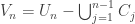 . Clearly each
  . It is straightforward to verify that
  is a cover of
  . Choose an open set
  . Then
  and
and  . This means that
  for all
  . Thus the open cover
  be an increasing open cover of
  of
of  . Then
  is also a locally finite refinement of
 if
if  for all
  . Then we have the following:
 be a decreasing sequence of closed subsets of
  for each
  . We claim that
  is a decreasing sequence of open sets that expand the closed sets
  . The expansion part follows from the following:

 for some
  . Since
  ,
,  . This in turns means that
  , a contradiction. Thus we have
  for some
![F \times [0,1]](https://s0.wp.com/latex.php?latex=F+%5Ctimes+%5B0%2C1%5D&bg=ffffff&fg=333333&s=0&c=20201002) , is a normal space.
, is a normal space.  be any uncountable set. Let
  many copies of the two element set
  . The usual notation of this product space is
  . The elements of
  that maps every subset of
  many subsets of the real line where
  such that
  .
.![f_0([0,1])=1](https://s0.wp.com/latex.php?latex=f_0%28%5B0%2C1%5D%29%3D1&bg=ffffff&fg=333333&s=0&c=20201002)
![f_0([1,2])=0](https://s0.wp.com/latex.php?latex=f_0%28%5B1%2C2%5D%29%3D0&bg=ffffff&fg=333333&s=0&c=20201002)


 . Members of
  are easy to describe. Each function in
  based on membership (whether the reference point belongs to the set
  ). Points not in
  and
and  are not in
  , there is an open set
  containing
 and that
  for any real number
  .
.  and
and  , with nonempty intersection.
  be any open set containing
  and
and  from
from  . If there are only countably many distinct sets
  can be separated by disjoint open sets. To see this, define the following two open sets
  in the product topology.


 and
and  . Furthermore,
  . This observation will be the basis for showing that Bing’s Example G is normal.
 with points in
  and
and  where
where 

 and
and  . Thus Bing’s Example G is a normal space.
 be the set of all open sets in
  . From the perspective of Bing’s Example G, the sets
  for each
  . Let
. Let  . Consider the following.
 . Any point that is not in one of the
  and each singleton set is contained in some member of
  are disjoint. Any point in