
This is another post Stone-Cech compactification. The links for other posts on Stone-Cech compactification can be found below. In this post, we prove a few basic facts about 


- The cardinality of
.
- The weight of
- The space
- Every infinite closed subset of
- The space
- No point of
is an isolated point.
- The space
- The space
- The space
- The space
- The space
- The space
- No point of the remainder
-point.
- The remainder
___________________________________________________________________________________
Characterization Theorems
For any completely regular space 

![I=[0,1]](https://s0.wp.com/latex.php?latex=I%3D%5B0%2C1%5D&bg=ffffff&fg=333333&s=0&c=20201002)

![[0,1]^{C(X,I)}](https://s0.wp.com/latex.php?latex=%5B0%2C1%5D%5E%7BC%28X%2CI%29%7D&bg=ffffff&fg=333333&s=0&c=20201002)
![\beta:X \rightarrow [0,1]^{C(X,I)}](https://s0.wp.com/latex.php?latex=%5Cbeta%3AX+%5Crightarrow+%5B0%2C1%5D%5E%7BC%28X%2CI%29%7D&bg=ffffff&fg=333333&s=0&c=20201002)
The brief sketch of 
-
_______________________________________________________________________________________
Theorem C1
Let
be a completely regular space. Let  be a continuous function from into a compact Hausdorff space
  . Then there is a continuous
  such that
  .
.

-
Theorem U1
If
 is any compactification of that satisfies condition in Theorem C1, then must be equivalent to .
See Two Characterizations of Stone-Cech Compactification.
_______________________________________________________________________________________
-
Theorem C2
Let
be a completely regular space. Among all compactifications of the space , the Stone-Cech compactification of the space is maximal with respect to the partial order  .
.
-
Theorem U2
The property in Theorem C2 is unique to
. That is, if, among all compactifications of the space , is maximal with respect to the partial order , then  .
.
See Two Characterizations of Stone-Cech Compactification.
_______________________________________________________________________________________
-
Theorem C3
Let
be a completely regular space. The space is  -embedded in its Stone-Cech compactification .
-
Theorem U3.1
Let
be a completely regular space. Let . Let be a compactification of such that each continuous  can be extended to a continuous
  . Then must be .
-
Theorem U3.2
If
is any compactification of that satisfies the property in Theorem C3 (i.e., is -embedded in ), then must be .
See C*-Embedding Property and Stone-Cech Compactification.
_______________________________________________________________________________________
The following discussion illustrates how we can use some of these characterizations theorem to obtain information about
___________________________________________________________________________________
Result 1 and Result 2
According to the previous post (Stone-Cech Compactification is Maximal), we have for any completely regular space 


Result 1 is established if we have 


From the same previous post (Stone-Cech Compactification is Maximal), it is shown that 


___________________________________________________________________________________
Result 3
A space is said to be zero-dimensional whenever it has a base consisting of open and closed sets. The proof that
-
Theorem 1
Let
be a normal space. If  and are disjoint closed subsets of , then and have disjoint closures in .
Proof of Theorem 1
Let ![g:X \rightarrow [0,1]](https://s0.wp.com/latex.php?latex=g%3AX+%5Crightarrow+%5B0%2C1%5D&bg=ffffff&fg=333333&s=0&c=20201002)


![G:\beta X \rightarrow [0,1]](https://s0.wp.com/latex.php?latex=G%3A%5Cbeta+X+%5Crightarrow+%5B0%2C1%5D&bg=ffffff&fg=333333&s=0&c=20201002)


-
Theorem 2
Let
be a completely regular space. Let be a closed and open subset of . Then  (the closure of in ) is also a closed and open set in .
Proof of Theorem 2
Let 
![\gamma:X \rightarrow [0,1]](https://s0.wp.com/latex.php?latex=%5Cgamma%3AX+%5Crightarrow+%5B0%2C1%5D&bg=ffffff&fg=333333&s=0&c=20201002)


![\Gamma:\beta X \rightarrow [0,1]](https://s0.wp.com/latex.php?latex=%5CGamma%3A%5Cbeta+X+%5Crightarrow+%5B0%2C1%5D&bg=ffffff&fg=333333&s=0&c=20201002)


-
Lemma 3
For every
 ,
,  (the closure of
  in ) is both closed and open in .
Note that Lemma 3 is a corollary of Theorem 2.
-
Lemma 4
Let
 be a set that is both closed and open in . Then
  where
where  .
.
Proof of Lemma 4
Let 


Proof of Result 3
Let 


We claim that 


It is now clear that 
___________________________________________________________________________________
Result 4 and Result 5
Result 5 is a corollary of Result 4. We first prove two lemmas before proving Result 4.
-
Lemma 5
For each infinite
, (the closure of in ) is a homeomorphic copy of and thus has cardinality .
Proof of Lemma 5
Let ![g:A \rightarrow [0,1]](https://s0.wp.com/latex.php?latex=g%3AA+%5Crightarrow+%5B0%2C1%5D&bg=ffffff&fg=333333&s=0&c=20201002)
![f:\omega \rightarrow [0,1]](https://s0.wp.com/latex.php?latex=f%3A%5Comega+%5Crightarrow+%5B0%2C1%5D&bg=ffffff&fg=333333&s=0&c=20201002)


![F:\beta \omega \rightarrow [0,1]](https://s0.wp.com/latex.php?latex=F%3A%5Cbeta+%5Comega+%5Crightarrow+%5B0%2C1%5D&bg=ffffff&fg=333333&s=0&c=20201002)

Note that the function ![G: \overline{A} \rightarrow [0,1]](https://s0.wp.com/latex.php?latex=G%3A+%5Coverline%7BA%7D+%5Crightarrow+%5B0%2C1%5D&bg=ffffff&fg=333333&s=0&c=20201002)

-
Lemma 6
For each countably infinite
 such that is relatively discrete, (the closure of in ) is a homeomorphic copy of and thus has cardinality .
Proof of Lemma 6
Let 


Let ![f:A \rightarrow [0,1]](https://s0.wp.com/latex.php?latex=f%3AA+%5Crightarrow+%5B0%2C1%5D&bg=ffffff&fg=333333&s=0&c=20201002)
![F:\overline{A} \rightarrow [0,1]](https://s0.wp.com/latex.php?latex=F%3A%5Coverline%7BA%7D+%5Crightarrow+%5B0%2C1%5D&bg=ffffff&fg=333333&s=0&c=20201002)
We first define ![w:\omega \rightarrow [0,1]](https://s0.wp.com/latex.php?latex=w%3A%5Comega+%5Crightarrow+%5B0%2C1%5D&bg=ffffff&fg=333333&s=0&c=20201002)
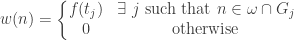
The function 


![W:\beta \omega \rightarrow [0,1]](https://s0.wp.com/latex.php?latex=W%3A%5Cbeta+%5Comega+%5Crightarrow+%5B0%2C1%5D&bg=ffffff&fg=333333&s=0&c=20201002)


Proof of Result 4
Let 


___________________________________________________________________________________
Result 6
We prove that no point in the remainder 


___________________________________________________________________________________
Result 7
The results under Result 7 are corollary of Result 5 (there is no non-trivial convergent sequence in
A space 


A space is said to be sequentially compact if every sequence of points in this space has a convergent subsequence. Even though
___________________________________________________________________________________
Result 8
Result 7.1 indicates that no point of remainder
___________________________________________________________________________________
Result 9
The space
There is a family 


For each 


___________________________________________________________________________________
Blog Posts on Stone-Cech Compactification
-
Post #0: Embedding Completely Regular Spaces into a Cube
Post #1: A Beginning Look at Stone-Cech Compactification
Post #2: Two Characterizations of Stone-Cech Compactification
Post #3: C*-Embedding Property and Stone-Cech Compactification
Post #4: Stone-Cech Compactification is Maximal
Post #5 (this post): Stone-Cech Compactification of the Integers – Basic Facts
Post #6: Stone-Cech Compactifications – Another Two Characterizations
___________________________________________________________________________________
Reference
- Engelking, R., General Topology, Revised and Completed edition, Heldermann Verlag, Berlin, 1989.
- Willard, S., General Topology, Addison-Wesley Publishing Company, 1970.
___________________________________________________________________________________

 , a subset of the square
  . An interesting property is when the diagonal of a space is a
  is said to be submetrizable if there is a topology
  that can be defined on
  is a metrizable space and
  . In other words, a submetrizable space is a space that has a coarser (weaker) metrizable topology. Every submetrizable space has a
  is always a
  is an infinite subset of
  , then
  is infinite for some
  (the set of all rational numbers). Let
  be the set of all irrational numbers. For each
  , choose a subsequence of
  consisting of distinct elements that converges to
  -space), denoted by
  . The underlying set is
  . Points in
  where
where  is finite. It is straightforward to verify that
  of open covers of a space
  and each open set
  with
with  such that any open set in
  containing the point
  . Clearly
  . Let
. Let  . For each
  for some
  . We claim that
  . Suppose that
  . By the definition of development, there exists some
  such that every open set in
  containing the point
  . Then
  , which contradicts
  . Thus we have
  .
. and let
  . The development is defined by
  , where for each
  consists of open sets of the form
  where
where  (
( ) that has not been covered by the sets
  spaces are defined using almost disjoint families, in our case, of subsets of
  is countably compact if every countable open cover of
  space. We also show that the converse does hold for normal spaces.
 be a family of infinite subsets of
  ,
,  is finite. The almost disjoint family
  is an infinite subset of
  , then
  is infinite for some
  .
. . To see this, identify
  (the set of all rational numbers). For each real number
  consisting of distinct elements that converges to
  . The underlying set is
  . Points in
  where
where  is finite. It is straightforward to verify that
  that is unbounded. We can find an infinite
  such that
  , then we have a contradiction since
  is a sequence that does not converge to
  . So we have
  is infinite for some
  is a sequence that does not converge to
  , another contradiction. So
  in
in  by
by  . According to the Tietze-Urysohn Theorem, in a normal space, any continuous function defined on a closed subset of
  , making
  of subsets of
  is a countable first countable space and is thus has a countable base (hence is normal). By Theorem 1, it is pseudocompact. By Theorem 2, it is countably compact. Yet