When two disjoint closed sets in a topological space cannot be separated by disjoint open sets, the space fails to be a normal space. When one of the two closed sets is countable, the space fails to satisfy a weaker property than normality. A space  is said to be a pseudonormal space if
  and
and  can always be separated by two disjoint open sets whenever and are disjoint closed subsets of and one of them is countable. In this post, we discuss several non-normal spaces that actually fail to be pseudonormal. We also give an example of a pseudonormal space that is not normal.
We work with spaces that are at minimum  spaces, i.e., spaces in which singleton sets are closed. Then any pseudonormal space is regular. To see this, let be and pseudonormal. For any closed subset
  of and for any point
  , we can always separate the disjoint closed sets
  and by disjoint open sets. This is one reason why we insist on having separation axiom as a starting point. We now show some examples of spaces that fail to be pseudonormal.
____________________________________________________________________
Some Non-Pseudonormal Examples
All three examples in this section are spaces where the failure of normality is exhibited by the inability of separating a countable closed set and another disjoint closed set.
Example 1
This example of a non-normal space that fails to be pseudonormal is defined in the previous post called An Example of a Completely Regular Space that is not Normal. This is an example of a Hausdorff, locally compact, zero-dimensional (having a base consisting of closed and open sets), metacompact, completely regular space that is not normal. We state the definition of the space and present a proof that it is not pseudonormal.
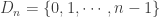
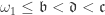
Let  be the set of all points
  such that
  . For each real number
  , define the following sets:
The set  is the vertical line of height 2 at the point
  . The set
  is the line originating at and going in the Northeast direction reaching the same vertical height as as shown in the following figure.
")
The topology on is defined by the following:
- Each point
 where
where  is isolated.
- For each point
 , a basic open set is of the form
  where
where  and
and  is a finite subset of
  .
.
The x-axis in this example is a closed and discrete set of cardinality continuum. Amy two disjoint subsets of the x-axis are disjoint closed sets. The two closed sets that cannot be separated are:
For each , let  where
where  is finite and
  . Furthermore, break up
  by letting
  and
and  . Let
. Let  and
and  be defined by:
The open sets  and
and  are essentially arbitrary open sets containing and respectively. We claims that
  .
.
Define the projection map  by
by  . Let
. Let  and
and  be defined by:
The set is countable. So the set is uncountable. Choose  . Choose
  on the left of and close enough to such that
  and
and  . This means that

 .
.
Thus . We have shown that the space is not pseudonormal and thus not normal.
Example 2
The Sorgenfrey line is the real line  topologized by the base consisting of half open and half closed intervals of the form
  . In this post, we use
  to denote the real line with this topology.
The Sorgenfrey line is a classic example of a normal space whose square  is not normal. In the Sorgenfrey plane , the set
  is a closed and discrete set and is called the anti-diagonal. The proof presented in this previous post shows that the following two disjoint closed subsets of
cannot be separated by disjoint open sets. The argument is based on the fact that the real line with the usual topology is of second category. The key point in the argument is that the set of the irrationals cannot be the union of countably many closed and nowhere dense sets (in the usual topology of the real line).
Thus fails to be pseudonormal. This example shows that normality can fail to be preserved by taking Cartesian product in such a way that even pseudonormality cannot be achieved in the Cartesian product!
Example 3
Another example of a non-normal space that fails to be pseudonormal is the Niemmytzkis’ plane (Example 2 in in this previous post). The underlying set is  . The points lying above the x-axis have the usual Euclidean open neighborhoods. A point in the x-axis has as neighborhoods
  together with the interior of a disc in the upper half plane that is tangent at the point . Consider the following the two disjoint closed sets on the x-axis:
The disjoint closed sets and cannot be separated by disjoint open sets (see Niemytzki’s Tangent Disc Topology in [2], Example 82). Like Example 2 above, the argument that and cannot be separated is also a Baire category argument.
____________________________________________________________________
An Example of Pseudonormal but not Normal
Example 4
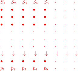
One way to find such a space is to look for spaces that are non-normal and see which one is pseudonormal. On the other hand, in a pseudonormal space, countable closed sets are easily separated from other disjoint closed sets. One space in which “countable” is nice is the first uncountable ordinal  with the order topology. But is normal. So we look at the Cartesian product
  . The second factor is the successor ordinal to or as a space that is obtained by tagging one more point to that is considered greater than all the points in . Let’s use
  to denote this space.
The space  is not normal (shown in this previous post). In the previous post, is presented as an example showing that the product of a normal space with a compact space needs not be normal. However, in this case at least, the product is pseudonormal.
Let  . Then the square
  as a subspace of is a countable space and a first countable space. So it has a countable base (second countable) and thus metrizable, and in particular normal. Any countable subset of is contained in one of these countable squares, making it easy to separate a countable closed set from another closed set.
Let and be disjoint closed sets in such that is countable. Then there is some successor ordinal  (
( for some ordinal
  ) such that
  . Based on the discussion in the preceding paragraph, there are disjoint open sets
  and
and  in
in  such that
  and
and  . With
  being a successor ordinal, the square is both closed and open in . Then the following sets
are disjoint open sets in separating and .
____________________________________________________________________
Some Comments about Examples 1 – 3
In each of Examples 1, 2 and 3 discussed above, there is a closed and discrete set of cardinality continuum (the x-axis in Examples 1 and 3 and the anti-diagonal in Example 2). So the extent of each of these three spaces is continuum. Note that the extent of a space is the maximum cardinality of a closed and discrete subset.
In each of these examples, it just so happens that it is not possible to separate the rationals from the irrationals in the x-axis or the anti-diagonal by disjoint open sets, making each example not only not normal but also not pseudonormal.
What if we consider a smaller subset of the x-axis or anti-diagonal? For example, consider an uncountable set of cardinality less than continuum. Then what can we say about the pseudonormality or normality of the resulting subspaces? For Example 1, the picture is clear cut.
In Example 1, the argument that and cannot be separated is a “countable vs. uncountable” argument. The argument will work as long as is a countable dense set in the x-axis (dense in the usual topology) and is any uncountable set.
For Example 2 and Example 3, the argument that and cannot be separated is not a “countable vs. uncountable” argument and instead is a Baire category argument. The fact that one of the closed sets is the irrationals is a crucial point. On the other hand, both Example 2 and Example 3 (especially Example 3) are set-theoretic sensitive examples. For Example 2 and Example 3, the normality of the resulting smaller subspaces is dependent on some extra axioms beyond ZFC. For pseudonormality, it could be set-theoretic sensitive too. We give some indication here why this is so.
Let be the Sorgenfrey line as in Example 2 above. Assuming Martin’s Axiom and the negation of the continuum hypothesis (abbreviated by MA + not CH), for any uncountable  with
with  ,
,  is normal but not paracompact (see Example 6.3 in [1] and see [3]). Even though is not exactly a comparable example, this example shows that restricting to a smaller subset on the anti-diagonal seems to make the space normal.
Example 3 has an illustrious history with respect to the normal Moore space conjecture. There is not surprise that extra set-theory axioms are used. For any subset of the x-axis, let  be the space defined as in Example 3 above except that only points of are used on the x-axis. Assuming MA + not CH, for any uncountable that is of cardinality less than continuum, it can be shown that is normal non-metrizable Moore space (see Example F in [4]). So by assuming extra axiom of MA + not CH, we cannot get a non-pseudonormal example out of Example 3 by restricting to a smaller uncountable subset of the x-axis. Under other set-theoretic axioms, there exists no normal non-metrizable Moore space. Just because this is a set-theoretic sensitive example, it is conceivable that could be a space that is not pseudonormal under some other axioms.
____________________________________________________________________
Reference
- Burke, D. K., Covering Properties, Handbook of Set-Theoretic Topology (K. Kunen and J. E. Vaughan, eds), Elsevier Science Publishers B. V., Amsterdam, 347-422, 1984.
- Steen, L. A., Seebach, J. A., Counterexamples in Topology, Dover Publications, Inc, Amsterdam, New York, 1995.
- Przymusinski, T. C., A Lindelof space such that is normal but not paracompact, Fund. Math., 91, 161-165, 1973.
- Tall, F. D., Normality versus Collectionwise Normality, Handbook of Set-Theoretic Topology (K. Kunen and J. E. Vaughan, eds), Elsevier Science Publishers B. V., Amsterdam, 685-732, 1984.
____________________________________________________________________


is made an isolated point.
 where
where 


 is the limit of the sequence
  . In this Euclidean space, the points in the sequences
 with the quotient topology. With the quotient topology, an open set containing the point
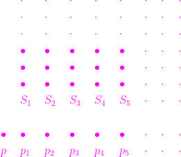
 consists of the point
  . Note that no sequence of points in
  is Frechet, all we need to do is to determine if
  . As observed in the preceding paragraph, no sequence of points in
  . This means that
  where the first factor
  is the product of continuum many copies of the unit interval
 ![I=[0,1]](https://s0.wp.com/latex.php?latex=I%3D%5B0%2C1%5D&bg=ffffff&fg=333333&s=0&c=20201002) .
. is not normal. This indicates that the result not shown in Steen and Seebach was because it was given as a problem and not because the tool for solving it was not yet available. The fact that it is given as an exercise also means that there is a more basic proof of the non-normality of
  is the immediate successor of
  with
with  . The ordinal
  and
and ![\omega_1+1=[0, \omega_1]](https://s0.wp.com/latex.php?latex=%5Comega_1%2B1%3D%5B0%2C+%5Comega_1%5D&bg=ffffff&fg=333333&s=0&c=20201002) . As ordinals,
. As ordinals, ![[0, \omega_1) \times [0, \omega_1]](https://s0.wp.com/latex.php?latex=%5B0%2C+%5Comega_1%29+%5Ctimes+%5B0%2C+%5Comega_1%5D&bg=ffffff&fg=333333&s=0&c=20201002) is a classic example of a product of a normal space (the first factor) and a compact space (the second factor) that is not normal. This example and others like it show that normality is easily broken upon taking product even if one of the factors is as nice as a compact space. The non-normality of
is a classic example of a product of a normal space (the first factor) and a compact space (the second factor) that is not normal. This example and others like it show that normality is easily broken upon taking product even if one of the factors is as nice as a compact space. The non-normality of 

![[0, \omega_1]](https://s0.wp.com/latex.php?latex=%5B0%2C+%5Comega_1%5D&bg=ffffff&fg=333333&s=0&c=20201002) can be embedded in the product space
can be embedded in the product space  , the product of
  . This means that
  as follows:
 by letting
  for all
  with
with  . The mapping is clearly one-to-one from
  . Upon closer inspection, the mapping in each direction is continuous (this is a good exercise to walk through). Thus, the mapping is a homeomorphism. It follows that
  , i.e., the Stone-Cech compactification of the first uncountable ordinal is its immediate successor.
 is bounded and is eventually constant (see result B
  , we can simply define
  to be the eventual constant value. A subspace
  -embedded in
 ![[0,\omega_1]](https://s0.wp.com/latex.php?latex=%5B0%2C%5Comega_1%5D&bg=ffffff&fg=333333&s=0&c=20201002) and
and  is normal.
 . See result G
  is not normal. The contrapositive statement would be the following:
 is normal, then
  but
but  for any countable
  , i.e., the last point is the limit point of the set of all the points preceding it but is not in the closure of any countable set. This means that the space
  . The set
  where each
  . As a product of compact spaces,
  is compact.
  for all
  (such a function is usually referred to as non-decreasing). Helly space is the subspace
  is normal.
 is Example 106 in [2]. This product is not normal. The non-normality of
  defined as follows:
 . Let
. Let 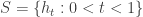 . Consider the mapping
  defined by
  . With the domain
  having the Sorgenfrey topology and with the range
  is a homeomorphism.

 is a closed subset of
  , define
  as follows:
 . The set
  ,
,  (closure taken in
  be a countable base for the usual topology on the unit interval


 and for each
  with
with  , we would like to arrange the elements in increasing order, notated as follow:
 . For the set
  ,
,  is to the left of
  for
for  . Note that elements of
  . If
. If  , then
  . If
. If  , then
 ![E_n=(p_n,q_n]=(p_n,1]](https://s0.wp.com/latex.php?latex=E_n%3D%28p_n%2Cq_n%5D%3D%28p_n%2C1%5D&bg=ffffff&fg=333333&s=0&c=20201002) .
. as follows:
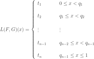
 when both
 be the set of
  is not hereditarily normal (see Theorem 3 in
  or
or  . In fact, for any compact non-metric space
  . In this post, we draw more continuous functions with the goal of connecting
  where
where ![D=[0,1] \times \{ 0,1 \}](https://s0.wp.com/latex.php?latex=D%3D%5B0%2C1%5D+%5Ctimes+%5C%7B+0%2C1+%5C%7D&bg=ffffff&fg=333333&s=0&c=20201002) , which is a subset in the Euclidean plane.
, which is a subset in the Euclidean plane. with
with  , a basic open set containing the point
  is of the form
 ![\displaystyle \biggl[ [a,b) \times \{ 1 \} \biggr] \cup \biggl[ (a,b) \times \{ 0 \} \biggr]](https://s0.wp.com/latex.php?latex=%5Cdisplaystyle+%5Cbiggl%5B+%5Ba%2Cb%29+%5Ctimes+%5C%7B+1+%5C%7D+%5Cbiggr%5D+%5Ccup+%5Cbiggl%5B+%28a%2Cb%29+%5Ctimes+%5C%7B+0+%5C%7D+%5Cbiggr%5D&bg=ffffff&fg=333333&s=0&c=20201002) , painted red in Figure 2. One the other hand, for any
, painted red in Figure 2. One the other hand, for any  , a basic open set containing the point
  is of the form
 ![\biggl[ (c,a) \times \{ 1 \} \biggr] \cup \biggl[ (c,a] \times \{ 0 \} \biggr]](https://s0.wp.com/latex.php?latex=%5Cbiggl%5B+%28c%2Ca%29+%5Ctimes+%5C%7B+1+%5C%7D+%5Cbiggr%5D+%5Ccup+%5Cbiggl%5B+%28c%2Ca%5D+%5Ctimes+%5C%7B+0+%5C%7D+%5Cbiggr%5D&bg=ffffff&fg=333333&s=0&c=20201002) , painted blue in Figure 2. The upper right point
, painted blue in Figure 2. The upper right point  and the lower left point
  are made isolated points.
![[0,1]](https://s0.wp.com/latex.php?latex=%5B0%2C1%5D&bg=ffffff&fg=333333&s=0&c=20201002) onto the upper line segment of the double arrow space, as demonstrated by the red arrow. Thus
onto the upper line segment of the double arrow space, as demonstrated by the red arrow. Thus  for any
  . Essentially on the interval
  onto the lower line segment of the double arrow space less the point
  , as demonstrated by the blue arrow in Figure 3. Thus
  for any
  with
with  . Essentially on the interval
 ![[-1,1]](https://s0.wp.com/latex.php?latex=%5B-1%2C1%5D&bg=ffffff&fg=333333&s=0&c=20201002) in the domain. To complete the mapping, let
in the domain. To complete the mapping, let  for any
  and
and  for any
  .
. be the mapping that has been described. It maps the Sorgenfrey line onto the double arrow space. It is straightforward to verify that the map
  is continuous.
 can be embedded into
  .
. for each
  . Thus each function
  where
where  is an embedding is shown in
 , let
, let  be the continuous function described in Figure 4.
  is a closed and discrete subspace of
  .
. , we define continuous functions
  such that
  . We can actually back out the map
  from
from  in Figure 4 and the mapping
  and
and  , where
  . So the function
 ![(a,1] \times \{ 0 \}](https://s0.wp.com/latex.php?latex=%28a%2C1%5D+%5Ctimes+%5C%7B+0+%5C%7D&bg=ffffff&fg=333333&s=0&c=20201002) . So
. So  and
and  , where
  . So the function
 ![(0,a] \times \{ 0 \}](https://s0.wp.com/latex.php?latex=%280%2Ca%5D+%5Ctimes+%5C%7B+0+%5C%7D&bg=ffffff&fg=333333&s=0&c=20201002) . So
. So ![\displaystyle U_a(y) = \left\{ \begin{array}{ll} \displaystyle 1 &\ \ \ \ \ \ y \in [a,1) \times \{ 1 \} \\ \text{ } & \text{ } \\ \displaystyle 1 &\ \ \ \ \ \ y \in (a,1] \times \{ 0 \} \\ \text{ } & \text{ } \\ 0 &\ \ \ \ \ \ y \in (0,a] \times \{ 0 \} \\ \text{ } & \text{ } \\ 0 &\ \ \ \ \ \ y \in [0,a) \times \{ 1 \} \\ \text{ } & \text{ } \\ 0 &\ \ \ \ \ \ y=(0,0) \text{ or } y = (1,1) \end{array} \right.](https://s0.wp.com/latex.php?latex=%5Cdisplaystyle++U_a%28y%29+%3D+%5Cleft%5C%7B+%5Cbegin%7Barray%7D%7Bll%7D+++++++++++%5Cdisplaystyle++1+%26%5C+%5C+%5C+%5C+%5C+%5C+y+%5Cin+%5Ba%2C1%29+%5Ctimes+%5C%7B+1+%5C%7D+%5C%5C++++++++++++%5Ctext%7B+%7D+%26+%5Ctext%7B+%7D+%5C%5C++++++++++%5Cdisplaystyle++1+%26%5C+%5C+%5C+%5C+%5C+%5C+y+%5Cin+%28a%2C1%5D+%5Ctimes+%5C%7B+0+%5C%7D+%5C%5C+++++++++++%5Ctext%7B+%7D+%26+%5Ctext%7B+%7D+%5C%5C+++++++++++0+%26%5C+%5C+%5C+%5C+%5C+%5C+y+%5Cin+%280%2Ca%5D+%5Ctimes+%5C%7B+0+%5C%7D+%5C%5C+++++++++++%5Ctext%7B+%7D+%26+%5Ctext%7B+%7D+%5C%5C+++++++++++0+%26%5C+%5C+%5C+%5C+%5C+%5C+y+%5Cin+%5B0%2Ca%29+%5Ctimes+%5C%7B+1+%5C%7D+%5C%5C+++++++++++%5Ctext%7B+%7D+%26+%5Ctext%7B+%7D+%5C%5C+++++++++++0+%26%5C+%5C+%5C+%5C+%5C+%5C+y%3D%280%2C0%29+%5Ctext%7B+or+%7D+y+%3D+%281%2C1%29+++++++++++%5Cend%7Barray%7D+%5Cright.&bg=ffffff&fg=333333&s=0&c=20201002)
 . Let
. Let  . The set
  -Theory Problem Book, Topological and Function Spaces, Springer, New York, 2011.
![F \times [0,1]](https://s0.wp.com/latex.php?latex=F+%5Ctimes+%5B0%2C1%5D&bg=ffffff&fg=333333&s=0&c=20201002) , is a normal space.
, is a normal space.  be the set of all subsets of
  many copies of the two element set
  . The usual notation of this product space is
  . The elements of
  many subsets of the real line where
  is the cardinality of the continuum.
  such that
  .
.![f_0([0,1])=1](https://s0.wp.com/latex.php?latex=f_0%28%5B0%2C1%5D%29%3D1&bg=ffffff&fg=333333&s=0&c=20201002)
![f_0([1,2])=0](https://s0.wp.com/latex.php?latex=f_0%28%5B1%2C2%5D%29%3D0&bg=ffffff&fg=333333&s=0&c=20201002)


 is the set of all irrational numbers. Consider the subspace
  . Members of
  are easy to describe. Each function in
  based on membership (whether the reference point belongs to the set
  ). Points not in
  and
and  are not in
  , there is an open set
  containing
 and that
  for any real number
  .
.  and
and  , with nonempty intersection.
  be any open set containing
  from
from  . If there are only countably many distinct sets
  can be separated by disjoint open sets. To see this, define the following two open sets
  and
and  in the product topology.


 and
and  . Furthermore,
  . This observation will be the basis for showing that Bing’s Example G is normal.
 with points in
  and
and  where
where 

 and
and  are disjoint open sets and that
  and
and  . Thus Bing’s Example G is a normal space.
 be a countable open cover of
  be the set of all open sets in
  , let
, let  . From the perspective of Bing’s Example G, the sets
  are discrete closed sets. In any normal space, countably many discrete closed sets can be separated by disjoint open sets (see Lemma 1
  be disjoint open sets such that
  for each
  . Let
. Let  . Consider the following.
 is an open cover of
  . Any point that is not in one of the
  and each singleton set is contained in some member of
  are disjoint. Any point in
 . The Sorgenfrey line is one of the most important counterexamples in general topology. One of the often recited facts about this counterexample is that the Sorgenfrey plane (the square of the Sorgengfrey line) is not normal. We show that, though far from normal, the Sorgenfrey plane is subnormal.
 of a space
  subset of
  subset of
  is a
is a  and
and  . A space
  and
and  of
of  and
and  . Clearly any normal space is subnormal. The Sorgenfrey plane is an example of a subnormal space that is not normal.
  show that these two weak forms of normality (pseudonormal and subnormal) are not equivalent. The space
  . The Sorgenfrey plane is the product space
  be the interior of
 where each
  is a closed subset of the real line
  . We claim that
  such that
  is a limit point of
  ,
,  for some
  . Note that
  , which means that no point of the open interval
  can belong to
  for some
  , a contradiction. Thus
 such that each
  , in addition to being a collection of basic open sets, is a discrete collection. The existence of such a base is equivalent to metrizability, a well known result called Bing’s metrization theorem (see Theorem 4.4.8 in [1]). Let
  , there is some open subset
  such that
  and
and  . Thus
  . Thus we have:
 , let
, let  be defined by
 , let
, let  where each
  is a closed subset of
  by
by
 . Since
  is discrete, there exists some open subset
  of
of  such that
  where
where  . Then
  is an open subset of
  such that
  . Then
  is a closed subset of
  over all countably many possible pairs
  . Thus
  and
and  where
where  and
and  are perfect. Also note that the Sorgenfrey plane topology is finer than the topologies for both
  . Consider the sets
  and
and  defined by:

 . We claim that
  , and for each positive integer
  , let
, let  be the half-open square
  . Then
  is a local base at the point
  by
by
 . We claim that each
  . In relation to the point


 , it follows that
  . We show that for each of these three sets, there is an open set containing the point
  . If
. If  . Let
. Let  . Note that
  and
and  . Now consider the following open set:
 . Suppose
  . Then
  and
and  . Consider the following set:
 , it follows that
  . Thus
  . It follows that
  since
since

 . Hence
  , a contradiction. Thus the claim that
  is symmetrical to the case
  . If
. If  . Let
. Let  . Note that
  and
and 
 . Suppose
  . Then
  and
and 
 . Thus the claim that
  is perfect, then
  is perfect. We take the inductive proof in [2] and adapt it for the Sorgenfrey plane. The authors in [2] also proved that for a sequence of spaces
  such that the product of any finite number of these spaces is perfect, the product
  is perfect. Then
  is perfect.
 with the order topology. Let
  be the disjoint sum (union) of
 be a pressing down function, i.e.,
  . Then there exists
  is a stationary set.
 . Suppose that
  where each
  is an open subset of
  . Then
  for some
  .
. is a limit, choose
  such that
 ![[g_n(\alpha),\alpha] \times [g_n(\alpha),\alpha] \subset O_n](https://s0.wp.com/latex.php?latex=%5Bg_n%28%5Calpha%29%2C%5Calpha%5D+%5Ctimes+%5Bg_n%28%5Calpha%29%2C%5Calpha%5D+%5Csubset+O_n&bg=ffffff&fg=333333&s=0&c=20201002) . The function
. The function  can be chosen since
  and there exists a stationary set
  such that
  for all
  . It follows that
  for each
  for all
  for each
  and
and  where each
  and each
  are open in
  , i.e.,
  for some
  such that
  is a successor ordinal. Note that
  . For each
  such that
 ![\left\{\beta \right\} \times [\delta_n,\omega_1] \subset V_n](https://s0.wp.com/latex.php?latex=%5Cleft%5C%7B%5Cbeta+%5Cright%5C%7D+%5Ctimes+%5B%5Cdelta_n%2C%5Comega_1%5D+%5Csubset+V_n&bg=ffffff&fg=333333&s=0&c=20201002) . Choose
. Choose  such that
  for all
  . Note that
  . It follows that
  . Thus there are no disjoint
  .
.![\mathcal{F}[\mathbb{R}]](https://s0.wp.com/latex.php?latex=%5Cmathcal%7BF%7D%5B%5Cmathbb%7BR%7D%5D&bg=ffffff&fg=333333&s=0&c=20201002) .
.