The preceding post is an exercise showing that the product of countably many  -compact spaces is a Lindelof space. The result is an example of a situation where the Lindelof property is countably productive if each factor is a “nice” Lindelof space. In this case, “nice” means -compact. This post gives several exercises surrounding the notion of -compactness.
Exercise 2.A
According to the preceding exercise, the product of countably many -compact spaces is a Lindelof space. Give an example showing that the result cannot be extended to the product of uncountably many -compact spaces. More specifically, give an example of a product of uncountably many -compact spaces such that the product space is not Lindelof.
Exercise 2.B
Any -compact space is Lindelof. Since ![\mathbb{R}=\bigcup_{n=1}^\infty [-n,n]](https://s0.wp.com/latex.php?latex=%5Cmathbb%7BR%7D%3D%5Cbigcup_%7Bn%3D1%7D%5E%5Cinfty+%5B-n%2Cn%5D&bg=ffffff&fg=333333&s=0&c=20201002) , the real line with the usual Euclidean topology is -compact. This exercise is to find an example of “Lindelof does not imply -compact.” Find one such example among the subspaces of the real line. Note that as a subspace of the real line, the example would be a separable metric space, hence would be a Lindelof space.
, the real line with the usual Euclidean topology is -compact. This exercise is to find an example of “Lindelof does not imply -compact.” Find one such example among the subspaces of the real line. Note that as a subspace of the real line, the example would be a separable metric space, hence would be a Lindelof space.
Exercise 2.C
This exercise is also to look for an example of a space that is Lindelof and not -compact. The example sought is a non-metric one, preferably a space whose underlying set is the real line and whose topology is finer than the Euclidean topology.
Exercise 2.D
Show that the product of two Lindelof spaces is a Lindelof space whenever one of the factors is a -compact space.
Exercise 2.E
Prove that the product of finitely many -compact spaces is a -compact space. Give an example of a space showing that the product of countably and infinitely many -compact spaces does not have to be -compact. For example, show that  , the product of countably many copies of the real line, is not -compact.
Comments
The Lindelof property and -compactness are basic topological notions. The above exercises are natural questions based on these two basic notions. One immediate purpose of these exercises is that they provide further interaction with the two basic notions. More importantly, working on these exercise give exposure to mathematics that is seemingly unrelated to the two basic notions. For example, finding -compactness on subspaces of the real line and subspaces of compact spaces naturally uses a Baire category argument, which is a deep and rich topic that finds uses in multiple areas of mathematics. For this reason, these exercises present excellent learning opportunities not only in topology but also in other useful mathematical topics.
If preferred, the exercises can be attacked head on. The exercises are also intended to be a guided tour. Hints are also provided below. Two sets of hints are given – Hints (blue dividers) and Further Hints (maroon dividers). The proofs of certain key facts are also given (orange dividers). Concluding remarks are given at the end of the post.

Hints for Exercise 2.A
Prove that the Lindelof property is hereditary with respect to closed subspaces. That is, if  is a Lindelof space, then every closed subspace of is also Lindelof.
Prove that if is a Lindelof space, then every closed and discrete subset of is countable (every space that has this property is said to have countable extent).
Show that the product of uncountably many copies of the real line does not have countable extent. Specifically, focus on either one of the following two examples.
- Show that the product space
 has a closed and discrete subspace of cardinality continuum where
  is cardinality of continuum. Hence is not Lindelof.
- Show that the product space
 has a closed and discrete subspace of cardinality
  where is the first uncountable ordinal. Hence is not Lindelof.
Hints for Exercise 2.B
Let  be the set of all irrational numbers. Show that as a subspace of the real line is not -compact.
Hints for Exercise 2.C
Let  be the real line with the topology generated by the half open and half closed intervals of the form
  . The real line with this topology is called the Sorgenfrey line. Show that is Lindelof and is not -compact.
Hints for Exercise 2.D
It is helpful to first prove: the product of two Lindelof space is Lindelof if one of the factors is a compact space. The Tube lemma is helpful.
Tube Lemma
Let be a space. Let  be a compact space. Suppose that
  is an open subset of
  and suppose that
  where
where  . Then there exists an open subset
  of such that
  .
.
Hints for Exercise 2.E
Since the real line  is homeomorphic to the open interval
  , is homeomorphic to
  . Show that is not -compact.
Further Hints for Exercise 2.A
The hints here focus on the example .
Let ![I=[0,1]](https://s0.wp.com/latex.php?latex=I%3D%5B0%2C1%5D&bg=ffffff&fg=333333&s=0&c=20201002) . Let
. Let  be the first infinite ordinal. For convenience, consider the set
  , the set of all non-negative integers. Since
  is a closed subset of
  , any closed and discrete subset of is a closed and discrete subset of . The task at hand is to find a closed and discrete subset of
  . To this end, we define
  after setting up background information.
For each  , choose a sequence
  of open intervals (in the usual topology of
  ) such that
 ,
, for each
  (the closure is in the usual topology of ).
Note. For each  , the open intervals
  are of the form
  . For
. For  , the open intervals are of the form
  . For
. For  , the open intervals are of the form
 ![(a,1]](https://s0.wp.com/latex.php?latex=%28a%2C1%5D&bg=ffffff&fg=333333&s=0&c=20201002) .
.
For each , define the map  as follows:
We are now ready to define . For each  ,
,  is the mapping
  defined by
  for each .
Show the following:
- The set has cardinality continuum.
- The set
 is a discrete space.
- The set is a closed subspace of .
Further Hints for Exercise 2.B
A subset  of the real line is nowhere dense in if for any nonempty open subset of , there is a nonempty open subset of such that
  . If we replace open sets by open intervals, we have the same notion.
Show that the real line with the usual Euclidean topology cannot be the union of countably many closed and nowhere dense sets.
Further Hints for Exercise 2.C
Prove that if and are -compact, then the product is -compact, hence Lindelof.
Prove that , the Sorgenfrey line, is Lindelof while its square  is not Lindelof.
Further Hints for Exercise 2.D
As suggested in the hints given earlier, prove that is Lindelof if is Lindelof and is compact. As suggested, the Tube lemma is a useful tool.
Further Hints for Exercise 2.E
The product space is a subspace of the product space ![[0,1]^\omega](https://s0.wp.com/latex.php?latex=%5B0%2C1%5D%5E%5Comega&bg=ffffff&fg=333333&s=0&c=20201002) . Since is compact, we can fall back on a Baire category theorem argument to show why cannot be -compact. To this end, we consider the notion of Baire space. A space is said to be a Baire space if for each countable family
. Since is compact, we can fall back on a Baire category theorem argument to show why cannot be -compact. To this end, we consider the notion of Baire space. A space is said to be a Baire space if for each countable family  of open and dense subsets of , the intersection
  is a dense subset of . Prove the following results.
Fact E.1
Let be a compact Hausdorff space. Let  be a sequence of non-empty open subsets of such that
  for each
  . Then the intersection
  is non-empty.
Fact E.2
Any compact Hausdorff space is Baire space.
Fact E.3
Let be a Baire space. Let be a dense  -subset of such that
  is a dense subset of . Then is not a -compact space.
Since ![X=[0,1]^\omega](https://s0.wp.com/latex.php?latex=X%3D%5B0%2C1%5D%5E%5Comega&bg=ffffff&fg=333333&s=0&c=20201002) is compact, it follows from Fact E.2 that the product space is a Baire space.
is compact, it follows from Fact E.2 that the product space is a Baire space.
Fact E.4
Let and  . The product space is a dense -subset of . Furthermore, is a dense subset of .
It follows from the above facts that the product space cannot be a -compact space.
Proofs of Key Steps for Exercise 2.A
The proof here focuses on the example .
To see that has the same cardinality as that of , show that  for
for  . This follows from the definition of the mapping .
To see that is discrete, for each , consider the open set  . Note that
  . Further note that
  for all
  .
.
To see that is a closed subset of , let  such that
  . Consider two cases.
Case 1.  for all
  .
.
Note that  is an open cover of (in the usual topology). There exists a finite
  such that
  is a cover of . Consider the open set
  . Define the set
  as follows:
The set can be further described as follows:
The last step is  because is a cover of . The fact that
  means that
  is an open subset of containing the point
  such that contains no point of .
Case 2.  for some .
Since ,  for all . In particular,
  . This means that
  for some . Define the open set as follows:
Clearly  . Observe that
  since
since  . For each
  ,
,  since
since  . Thus is an open set containing such that
  .
.
Both cases show that is a closed subset of .
Proofs of Key Steps for Exercise 2.B
Suppose that , the set of all irrational numbers, is -compact. That is,  where each
  is a compact space as a subspace of . Any compact subspace of is also a compact subspace of . As a result, each is a closed subset of . Furthermore, prove the following:
Each is a nowhere dense subset of .
Each singleton set  where
where  is any rational number is also a closed and nowhere dense subset of . This means that the real line is the union of countably many closed and nowhere dense subsets, contracting the hints given earlier. Thus cannot be -compact.
Proofs of Key Steps for Exercise 2.C
The Sorgenfrey line is a Lindelof space whose square is not normal. This is a famous example of a Lindelof space whose square is not Lindelof (not even normal). For reference, a proof is found here. An alternative proof of the non-normality of uses the Baire category theorem and is found here.
If the Sorgenfrey line is -compact, then would be -compact and hence Lindelof. Thus cannot be -compact.
Proofs of Key Steps for Exercise 2.D
Suppose that is Lindelof and that is compact. Let  be an open cover of . For each , let
  be finite such that
  is a cover of
  . Putting it another way,
  . By the Tube lemma, for each , there is an open
  such that
  . Since is Lindelof, there exists a countable set
  such that
  is a cover of . Then
  is a countable subcover of . This completes the proof that is Lindelof when is Lindelof and is compact.
To complete the exercise, observe that if is Lindelof and is -compact, then is the union of countably many Lindelof subspaces.
Proofs of Key Steps for Exercise 2.E
Proof of Fact E.1
Let be a compact Hausdorff space. Let be a sequence of non-empty open subsets of such that $latex for each . Show that the intersection is non-empty.
Suppose that  . Choose
  . There must exist some
  such that
  . Choose
  . There must exist some
  such that
  . Continue in this manner we can choose inductively an infinite set
  such that
  for
for  . Since is compact, the infinite set has a limit point
  . This means that every open set containing contains some
  (in fact for infinitely many ). The point cannot be in the intersection . Thus for some ,
  . Thus
  . We can choose an open set such that
  and
and  . However, must contain some point where
  . This is a contradiction since
  for all . Thus Fact E.1 is established.
Proof of Fact E.2
Let be a compact space. Let  be open subsets of such that each
  is also a dense subset of . Let a non-empty open subset of . We wish to show that contains a point that belongs to each . Since
  is dense in ,
  is non-empty. Since
  is dense in , choose non-empty open
  such that
  and
and  . Since
  is dense in , choose non-empty open
  such that
  and
and  . Continue inductively in this manner and we have a sequence of open sets just like in Fact E.1. Then the intersection of the open sets
  is non-empty. Points in the intersection are in and in all the
  . This completes the proof of Fact E.2.
Proof of Fact E.3
Let be a Baire space. Let be a dense -subset of such that is a dense subset of . Show that is not a -compact space.
Suppose is -compact. Let  where each
  is compact. Each is obviously a closed subset of . We claim that each is a closed nowhere dense subset of . To see this, let be a non-empty open subset of . Since is dense in , contains a point where
  . Since
  , there exists a non-empty open
  such that
  . This shows that each is a nowhere dense subset of .
Since is a dense -subset of ,  where each is an open and dense subset of . Then each
  is a closed nowhere dense subset of . This means that is the union of countably many closed and nowhere dense subsets of . More specifically, we have the following.
(1)………
Statement (1) contradicts the fact that is a Baire space. Note that all  and
and  are open and dense subsets of . Further note that the intersection of all these countably many open and dense subsets of is empty according to (1). Thus cannot not a -compact space.
Proof of Fact E.4
The space is compact since it is a product of compact spaces. To see that is a dense -subset of , note that  where for each integer
(2)………![U_n=(0,1) \times \cdots \times (0,1) \times [0,1] \times [0,1] \times \cdots](https://s0.wp.com/latex.php?latex=U_n%3D%280%2C1%29+%5Ctimes+%5Ccdots+%5Ctimes+%280%2C1%29+%5Ctimes+%5B0%2C1%5D+%5Ctimes+%5B0%2C1%5D+%5Ctimes+%5Ccdots&bg=ffffff&fg=333333&s=0&c=20201002)
Note that the first factors of are the open interval and the remaining factors are the closed interval ![[0,1]](https://s0.wp.com/latex.php?latex=%5B0%2C1%5D&bg=ffffff&fg=333333&s=0&c=20201002) . It is also clear that is a dense subset of . This completes the proof of Fact E.4.
. It is also clear that is a dense subset of . This completes the proof of Fact E.4.
Concluding Remarks
Exercise 2.A
The exercise is to show that the product of uncountably many -compact spaces does not need to be Lindelof. The approach suggested in the hints is to show that  has uncountable extent where is continuum. Having uncountable extent (i.e. having an uncountable subset that is both closed and discrete) implies the space is not Lindelof. The uncountable extent of the product space is discussed in this post.
For and , there is another way to show non-Lindelof. For example, both product spaces are not normal. As a result, both product spaces cannot be Lindelof. Note that every regular Lindelof space is normal. Both product spaces contain the product  as a closed subspace. The non-normality of is discussed here.
Exercise 2.B
The hints given above is to show that the set of all irrational numbers, , is not -compact (as a subspace of the real line). The same argument showing that is not -compact can be generalized. Note that the complement of is  , the set of all rational numbers (a countable set). In this case, is a dense subset of the real line and is the union of countably many singleton sets. Each singleton set is a closed and nowhere dense subset of the real line. In general, we can let
  , the complement of a set , be dense in the real line and be the union of countably many closed nowhere dense subsets of the real line (not necessarily singleton sets). The same argument will show that cannot be a -compact space. This argument is captured in Fact E.3 in Exercise 2.E. Thus both Exercise 2.B and Exercise 2.E use a Baire category argument.
Exercise 2.E
Like Exercise 2.B, this exercise is also to show a certain space is not -compact. In this case, the suggested space is  , the product of countably many copies of the real line. The hints given use a Baire category argument, as outlined in Fact E.1 through Fact E.4. The product space is embedded in the compact space
 ![[0,1]^{\omega}](https://s0.wp.com/latex.php?latex=%5B0%2C1%5D%5E%7B%5Comega%7D&bg=ffffff&fg=333333&s=0&c=20201002) , which is a Baire space. As mentioned earlier, Fact E.3 is essentially the same argument used for Exercise 2.B.
, which is a Baire space. As mentioned earlier, Fact E.3 is essentially the same argument used for Exercise 2.B.
Using the same Baire category argument, it can be shown that  , the product of countably many copies of the countably infinite discrete space, is not -compact. The space of the non-negative integers, as a subspace of the real line, is certainly -compact. Using the same Baire category argument, we can see that the product of countably many copies of this discrete space is not -compact. With the product space , there is a connection with Exercise 2.B. The product is homeomorphic to . The idea of the homeomorphism is discussed here. Thus the non--compactness of can be achieved by mapping it to the irrationals. Of course, the same Baire category argument runs through both exercises.
Exercise 2.C
Even the non--compactness of the Sorgenfrey line can be achieved by a Baire category argument. The non-normality of the Sorgenfrey plane can be achieved by Jones’ lemma argument or by the fact that is not a first category set. Links to both arguments are given in the Proof section above.
See here for another introduction to the Baire category theorem.
The Tube lemma is discussed here.
Dan Ma topology
Daniel Ma topology
Dan Ma math
Daniel Ma mathematics
 2019 – Dan Ma


.


continuum. The statement
.


![\{ [s]: \exists \ n \in \omega \text{ such that } s \in 2^n \}](https://s0.wp.com/latex.php?latex=%5C%7B+%5Bs%5D%3A+%5Cexists+%5C+n+%5Cin+%5Comega+%5Ctext%7B+such+that+%7D+s+%5Cin+2%5En+%5C%7D&bg=ffffff&fg=333333&s=0&c=20201002)
![[s]=\{ t \in 2^\omega: s \subset t \}](https://s0.wp.com/latex.php?latex=%5Bs%5D%3D%5C%7B+t+%5Cin+2%5E%5Comega%3A++s+%5Csubset+t+%5C%7D&bg=ffffff&fg=333333&s=0&c=20201002)
for any
.
, then
.

,
.


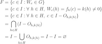
![[t] \cap C_i=\varnothing](https://s0.wp.com/latex.php?latex=%5Bt%5D+%5Ccap+C_i%3D%5Cvarnothing&bg=ffffff&fg=333333&s=0&c=20201002)


![[t] \cap C_0=\varnothing](https://s0.wp.com/latex.php?latex=%5Bt%5D+%5Ccap+C_0%3D%5Cvarnothing&bg=ffffff&fg=333333&s=0&c=20201002)


 such that for all
  ,
,  .
.


![[s]](https://s0.wp.com/latex.php?latex=%5Bs%5D&bg=ffffff&fg=333333&s=0&c=20201002)

![[s] \cap C(h)](https://s0.wp.com/latex.php?latex=%5Bs%5D+%5Ccap+C%28h%29&bg=ffffff&fg=333333&s=0&c=20201002)
![[t] \cap C_n=\varnothing](https://s0.wp.com/latex.php?latex=%5Bt%5D+%5Ccap+C_n%3D%5Cvarnothing&bg=ffffff&fg=333333&s=0&c=20201002)
![[t] \cap C(h) \ne \varnothing](https://s0.wp.com/latex.php?latex=%5Bt%5D+%5Ccap+C%28h%29+%5Cne+%5Cvarnothing&bg=ffffff&fg=333333&s=0&c=20201002)


 such that the product of
  ).
). be the Michael line. Let
  is not normal (see
  is not normal.
 . The set
  that is of first category in the real line,
  is at most countable. The Russian mathematician Luzin in 1914 constructed such an uncountable Luzin set using continuum hypothesis (CH). A good reference for Luzin sets is [4]. We have the following theorem.
 be the set of all closed nowhere dense sets in the real line. Choose a real number
  to start. For each
  with
with  , choose a real number
  not in the following set:
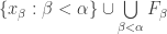
 . Then
  is a Luzin set.
 contains all but countably many points of
  are closed nowhere dense subsets of the real line, then
  contains all but countably many points of the Luzin set
  of the real line,
  be uncountable and dense in the real line such that
  is uncountable. Given a dense
  can only contain countably many points of
  where each
  is open and dense in
  , let
, let  . Each
  contains all but countably many points of the Luzin set
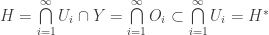
 . Then
  cannot be an
  -set in the Euclidean space
  be a countable dense subset of the real line. The set
  if for every open subset
  of the real line such that
  ,
,  . It is clear that adding countably many points to a Luzin set still results in a Luzin set. Thus
  are discrete and points in
  is dense in the real line.
 , the set of all rational numbers. Let
  be the usual topology of the real line
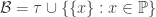
 is called the Michael line and is denoted by
  , the product
  is paracompact.
 is not normal.
 is not normal.
 of
of  . Let
. Let  . Note that
  such that
  is a locally finite open refinement
  and such that
  where
where  and let
  be an uncountable Euclidean closed set consisting entirely of irrational numbers. Then this set
  such that every closed and discrete set in
  . The extent of the space
  . When the cardinal number
  (the first infinite cardinal number), the space
  , there are uncountable closed and discrete subsets in the space.
 .
.  that is defined by
  . If the space is Hausdorff, the diagonal is always a closed set in the square. If
  is a
is a  be defined by the following:
 .
.
 and
and  where
where  with
with  . By
. By  , we mean
  . For each
  , choose an open interval
  such that
  . We also assume that
  is the midpoint of the open interval
  . For each positive integer
  be defined by:
 . For each
  (Euclidean closure in the real line). It is clear that
  . On the other hand,
  (otherwise
  such that
  . So choose a rational number
  .
. . Since
  such that
  . Now we have
  . Choose another integer
  such that
  and
and  .
. . Now it is clear that
  . The following inequalities show that
  .
.
 . Since
  ,
,  . Thus
  . We have shown that
  . Thus
  . The first
  is discrete (a subspace of the Michael line) and the second
  , choose
  such that
  . We can assume that
  where
where  .
. , choose some
  such that
  . We can assume that
  where
where  .
. is metacompact. So there is a point-finite open refinement
  of
of  . For each
  has a point-finite open refinement
  . Let
. Let  ,
,  . Thus, metacompactness is the best we can hope for.
 is the set of all Euclidean open intervals with rational endpoints. One reason for the interest in point-countable base is that any countable compact space (hence any compact space) with a point-countable base is metrizable (see
  of open and dense subsets of
  is dense in
  of subsets of a space
  such that
  and
and  is a dense set in
 where
where  .
.  . Since
  can be a nowhere dense set. Thus for some
  .
. . Since
  , let
, let  be the
  . Note that
  . Observe that
  and
and  is immediate.
 where each
  is nowhere dense in
  ,
, . Clearly,
  . Choose
  . Since
  and such that
  , say only up to
  (so
(so  for all
  ).
). are nowhere dense. So we can choose some open set
  such that
  misses the nowhere dense set
  . In particular, this means that
  , contradicting that
  be a metric space. Then the following conditions are equivalent.
 of non-empty closed subsets of
  .
. consisting of non-empty closed subsets of
  is a family of non-empty open subsets of
  for each
  .
. is a family of non-empty open subsets of
  .
. is dense in
  . We find open
  and
and  . Then we have a decreasing sequence of open sets
  . It is clear that
  .
.  . They take turn choosing nested decreasing nonempty open subsets of
  of
of  . At the nth play where
  and
and  . The player
  . Otherwise the player
  is a complete metric space, and hence is a Baire space. The space of irrational numbers
  intersect with every uncountable closed subset of the real line. We present an algorithm on how to generate such a set. Bernstein sets are not Lebesgue measurable. Our goal here is to show that Bernstein sets are Baire spaces but not weakly
  . The set
 ![[-b,b]](https://s0.wp.com/latex.php?latex=%5B-b%2Cb%5D&bg=ffffff&fg=333333&s=0&c=20201002) for
for  ). Thus we can say that there are exactly continuum many uncountable closed subsets of the real line.
  . By Lemma 1, each
  has cardinality
  be this well ordering.
 and
and  be the first two elements of
  . Let
. Let  and
and  be the first two elements of
  (based on
  and that for each
  , points
  and
and  have been selected. Then
  is nonempty since
  be the first two points of
  .
. . Then
  be a set of first category in
  contains a dense
  where each
  is a dense
 be the interior of the set
  . In particular,
  . Let
. Let  denote the collection of all functions
  . Identify each
  by the sequence
  . This identification makes notations in the proofs of Lemma 4 and Lemma 7 easier to follow. For example, for
  denotes a closed interval
  . When we choose two disjoint subintervals of this interval, they are denoted by
  and
and  . For
. For  refers to
  ,
,  refers to the sequence
  , and
, and  refers to the sequence
  and so on.
 . Let
. Let  .
. contains a Cantor set (hence an uncountable closed subset of the real line).
 where each
 ![I_\varnothing=[a,b] \subset O_0 \cap U](https://s0.wp.com/latex.php?latex=I_%5Cvarnothing%3D%5Ba%2Cb%5D+%5Csubset+O_0+%5Ccap+U&bg=ffffff&fg=333333&s=0&c=20201002) . Let
. Let  . Then pick two disjoint closed intervals
  and
and  such that they are subsets of the interior of
  and such that the lengths of both intervals are less than
  . Let
. Let  .
. step, suppose that all closed intervals
  and
and  such that each one is subset of
  . Let
. Let  over all
  is a Cantor set that is contained in
  . If
. If  contains an uncountable closed subset of
  such that
  be an open subset of
  . We have
  where each
  contains
  . This uncountable closed set
  .
. be a winning strategy for player
  . Let
. Let  by using the winning strategy
 ![I_{-1}=[a,b]](https://s0.wp.com/latex.php?latex=I_%7B-1%7D%3D%5Ba%2Cb%5D&bg=ffffff&fg=333333&s=0&c=20201002) . Let
. Let  . Let
. Let  and
and  . We take
  as the first move by the player
  . Let
. Let  .
. and
and  that are subsets of the interior of
  such that the lengths of these two intervals are less than
  and such that
  and
and  satisfy further properties, which are that
  and
and  are open in
  and
and  . Let
. Let  have been chosen. Then for each
  , and:
 and
and  ,
, and
and  are open in
  and
and 
 and
and  as two possible new moves by player

 .
. , which is a Cantor set, hence an uncountable subset of the real line. We claim that
  .
. . There there is some
  such that
  . The closed intervals
  are associated with a play of the Banach-Mazur game on
 must be nonempty. Thus
  .
. , and since the lengths of
  for some
  . It also follows that
  . Thus
  of open and dense subsets of
  is dense in
  , then this sequence of open sets is said to be a play of the game.
 . In either version, the goal of player
  where each
  is nowhere dense in
  .
. (the first move) and for each partial play of the game (
 ,
, is a nonempty open set such that
  above,
  .
.
 and player
  ,
, is a nonempty open set such that
  be a nonempty open set. Let
  be a function such that for each
  ,
,  . Then there exists a disjoint collection
  such that
  is dense in
  be the set consisting of all collections
  . To see this, let
  and
and  . This is possible since
  . Then we have
  . Order
  is a partially ordered set.
  be a chain (a totally ordered set). We wish to show that
  has an upper bound in
  since it is clear that for each
  ,
,  . We only need to show
  . To this end, we need to show that any two elements of
  . Then
  and
and  for some
  and
and  . Since
  or
or  . This means that
  and
and  belong to the same disjoing collection in
  ,
,  Suppose that
  such that
  where each
  if
if  is the last move by
  Suppose that
  . Apply Lemma 1 to obtain a disjoint collection
  consisting of open sets of the form
  such that
  is dense in
  , we have
  for all open
  . So the function
  is like the function
  in Lemma 1. We can then apply Lemma 1 to obtain a disjoint collection
  consisting of open sets of the form
  such that
  is dense in
  . Based on how
  is dense in
  consisting of open sets of the form
  (these are moves made by
  is dense in
  . Each
  . From this nonempty intersection, we can extract a play of the game such that the open sets in this play of the game have one point in common (i.e. player
  is a strategy for
  , the strategy
  . A space
 . The intersection
  is dense in
  . Let
. Let  is dense in
  such that
  and
and  with the additional condition that the diameter of
  is less than
  .
. is dense in
  such that
  and
and  with the additional condition that the diameter of
  is less than
  .
. and a sequence of points
  such that
  for each
  converge to zero (according to some complete metric on
  . To see this, note that for each
  for each
  . Since
  for each
  for each
  ) and
) and  . This completes the proof of Baire category theorem.
  .
.  . For each
  . Then each
  is an open and dense set in
  .
. whose intersection is empty. Note that any point that belongs to all
  is a topological space such that for each countable family
  is dense in
  ). A set
  is nowhere dense in
  is nowhere dense in
  is an open and dense set in
  ,
, ![T=[0,1] \cup (\mathbb{Q} \cap [2,3])](https://s0.wp.com/latex.php?latex=T%3D%5B0%2C1%5D+%5Ccup+%28%5Cmathbb%7BQ%7D+%5Ccap+%5B2%2C3%5D%29&bg=ffffff&fg=333333&s=0&c=20201002) . The space
. The space  is not a Baire space since after taking away the rational numbers in
 ![[2,3]](https://s0.wp.com/latex.php?latex=%5B2%2C3%5D&bg=ffffff&fg=333333&s=0&c=20201002) , the remainder is no longer dense in
, the remainder is no longer dense in  . Theorems 2 and 1a indicate that any Baire space is of second category in itself. The converse is not true (see the space
  where each
  such that
  where each
  is nowhere dense in
  such that
  . Note that for each
  is closed and nowhere dense in