Perfect preimages of Lindelof spaces

Posted on April 7, 2023 by Dan Ma

Let $f:X \rightarrow Y$ be a mapping from a topological space $X$ onto a topological space $Y$ . If $f$ is a perfect map and $Y$ is a Lindelof space, then so is $X$ . If $f$ is a closed map and $Y$ is a paracompact space, then so is $X$ . In other words, the pre-image of a Lindelof space under a perfect map is always a Lindelof space. Likewise, the pre-image of a paracompact space under a closed map is always a paracompact space. After proving these two facts, we show that for any compact space $Y$ , the product $X \times Y$ is Lindelof (paracompact) for any Lindelof (paracompact) space $X$ . All spaces under consideration are Hausdorff.

Another way to state the above two facts is that Lindelofness is an inverse invariance under perfect maps and that paracompactness is an inverse invariance of the closed maps. In general, a topological property is an inverse invariance of a class of mappings $\mathcal{M}$ if the following holds: for any mapping $f:X \rightarrow Y$ belonging to $\mathcal{M}$ , if $Y$ has the property, then so does $X$ . In contrast, a topological property is an invariance of a class of mappings $\mathcal{M}$ if for any mapping $f:X \rightarrow Y$ belonging to $\mathcal{M}$ , if $X$ has the property, then so does $Y$ .

All mappings under consideration are continuous maps. A mapping $f:X \rightarrow Y$ , where $f(X)=Y$ , is a closed map if for any closed subset $A$ of $X$ , $f(A)$ is closed in $Y$ . A mapping $f:X \rightarrow Y$ , where $f(X)=Y$ , is a perfect map if $f$ is a closed map and that the point inverse $f^{-1}(y)$ is compact for each $y \in Y$ .

Perfect mappings and closed mappings are objects with strong properties. Such a map places a restriction on what topological properties the “domain” space or the “range” space can have. The theorems below indicate that it is not possible to map a non-Lindelof space onto a Lindelof space using a perfect map and that it is not possible to map a non-paracompact space onto a paracompact space using a closed map. On the other hand, it is not possible to map a separable metric space onto a separable but non-metric space using a perfect map (see here). We prove the following theorems.

Theorem 1…. Lindelofness (or the Lindelof property) is an inverse invariant of the perfect maps.

Theorem 2 ….Paracompactness is an inverse invariant of the closed maps.

Lemma 3 …. Let $f:X \longrightarrow Y$ be a closed map with $f(X)=Y$ . Let $V$ be an open subset of $X$ . Define $f_*(V)=\{ y \in Y: f^{-1}(y) \subset V \}$ . Then the set $f_*(V)$ is open in $Y$ and that $f_*(V) \subset f(V)$ .

For the proof of Lemma 3, see Lemma 2 here.

Proof of Theorem 1
Let $f:X \longrightarrow Y$ be a perfect map with $f(X)=Y$ . Suppose $Y$ is Lindelof. Let $\mathcal{U}$ be an open cover of $X$ . Without loss of generality, we can assume that $\mathcal{U}$ is closed under finite unions. For each $U \in \mathcal{U}$ , define $f_*(U)=\{ y \in Y: f^{-1}(y) \subset U \}$ . By Lemma 3, each $f_*(U)$ is an open subset of $Y$ . We claim that $\mathcal{V}=\{ f_*(U): U \in \mathcal{U} \}$ is an open cover of $Y$ . To this end, let $y \in Y$ . Since $f$ is a perfect map, the point inverse $f^{-1}(y)$ is compact. As a result, we can find a finite $\mathcal{F} \subset \mathcal{U}$ such that $f^{-1}(y) \subset \bigcup \mathcal{F}=W$ . Since $\mathcal{U}$ is closed under finite unions, $W \in \mathcal{U}$ . It follows that $y \in f_*(W)$ . Since $Y$ is Lindelof, there exists a countable $\{W_0,W_1,W_2,\cdots \} \subset \mathcal{V}$ such that $Y = \bigcup_{n=0}^\infty W_n$ . For each $n$ , $W_n=f_*(U_n)$ for some $U_n \in \mathcal{U}$ . We claim that $\{U_0,U_1,U_2,\cdots \}$ is a cover of $X$ . To this end, let $x \in X$ . Then for some $n$ , $y=f(x) \in W_n=f_*(U_n)$ . This implies that $x \in f^{-1}(y) \subset U_n$ . Thus, the open cover $\mathcal{U}$ has a countable subcover. This concludes the proof of Theorem 1. $\square$

Proof of Theorem 2
Let $f:X \longrightarrow Y$ be a perfect map with $f(X)=Y$ . Suppose $Y$ is paracompact. Let $\mathcal{U}$ be an open cover of $X$ . For each $U \in \mathcal{U}$ , define $f_*(U)$ as in Lemma 3. By Lemma 3, each $f_*(U)$ is an open subset of $Y$ . Let $\mathcal{V}=\{ f_*(U): U \in \mathcal{U} \}$ . As shown in the proof of Theorem 1, $\mathcal{V}$ is an open cover of $Y$ . Since $Y$ is paracompact, there exists a locally finite open refinement $\mathcal{W}$ of $\mathcal{V}$ . Let $\mathcal{W}_0=\{ f^{-1}(W): W \in \mathcal{W} \}$ .

We show three facts about $\mathcal{W}_0$ . (1) It is an open cover of $X$ . (2) It is a locally finite collection in $X$ . (3) It is a refinement of $\mathcal{U}$ . To see (1), note that $\mathcal{W}$ is an open cover of $Y$ . As a result, $\mathcal{W}_0$ is an open cover of $X$ . To see (2), let $x \in X$ . We find an open $O \subset X$ such that $x \in O$ and such that $O$ intersects only finitely many elements of $\mathcal{W}_0$ . Since $\mathcal{W}$ is locally finite in $Y$ , there exists an open $B \subset Y$ such that $y=f(x) \in B$ and such that $B$ intersects only finitely many elements of $\mathcal{W}$ , say, $W_0,W_1,\cdots,W_n$ . Let $O=f^{-1}(B)$ . Clearly, $x \in O$ . It can be verified that the only elements of $\mathcal{W}_0$ having non-empty intersections with $O$ are $f^{-1}(W_0)$ , $f^{-1}(W_1),\cdots$ , $f^{-1}(W_n)$ . To see (3), let $f^{-1}(W) \in \mathcal{W}_0$ where $W \in \mathcal{W}$ . Then $W \subset V=f_*(U)$ for some $V \in \mathcal{V}$ and some $U \in \mathcal{U}$ . We claim that $f^{-1}(W) \subset U$ . Let $x \in f^{-1}(W)$ . Then $y=f(x) \in W \subset V=f_*(U)$ . This implies that $x \in f^{-1}(y) \subset U$ . It follows that $\mathcal{W}_0$ is a locally finite open refinement of the open cover $\mathcal{U}$ . This completes the proof of Theorem 2. $\square$

Productively Paracompact Spaces

A space $X$ is productively paramcompact if $X \times Y$ is paracompact for every paracompact space $Y$ . The definition for productively Lindelof can be stated in a similar way. For some reason, the term “productively paracompact” is not used in the literature but is a topic that had been extensively studied. It is also a topic found in this site. The following four classes of spaces are productively paracompact (see here and here).

Compact spaces
$\sigma$ -compact spaces
Locally compact spaces
$\sigma$ -locally compact spaces

The proof for compact spaces being productively paracompact given here uses the Tube Lemma (see here). As applications of Theorem 1 and Theorem 2, we use the two theorems to show that compact spaces are both productively Lindelof and productive paracompact.

Theorem 4…. Let $Y$ any compact space. Then $X \times Y$ is Lindelof for every Lindelof space $X$ .

Theorem 5 ….Let $Y$ any compact space. Then $X \times Y$ is paracompact for every paracompact space $X$ .

Theorems 4 and 5 are corollaries to the Kuratowski theorem (see here) and Theorems 1 and 2 above. Suppose $Y$ is compact. Then the projection map from $X \times Y$ onto $X$ is a closed map. The paracompactness of $X \times Y$ follows whenever $X$ is paracompact. The projection map is also perfect since the point inverses are compact due to the compactness of the factor $Y$ . Then the Lindelofness of $X \times Y$ follows whenever $X$ is Lindelof.

$\text{ }$

Dan Ma invariant
Daniel Ma invariant

Dan Ma Inverse invariant
Daniel Ma Inverse invariant

Dan Ma perfect map
Daniel Ma perfect map

Dan Ma paracompact space
Daniel Ma paracompact space

Dan Ma Lindelof space
Daniel Ma Lindelof space

Dan Ma topology
Daniel Ma topology

$\copyright$ 2023 – Dan Ma

A Pixley-Roy Meta-Lindelof Space

Posted on November 1, 2022 by Dan Ma

The discussion in the preceding post pointed to a natural question of whether we have a theorem of CCC + meta-Lindelof $\rightarrow$ Lindelof or there is a counterexample. In this post, we present a counterexample. The example is a Pixley-Roy hyperspace $\mathcal{F}[X]$ , which is always metacompact, hence meta-Lindelof. We then make sure the ground $X$ is chosen appropriately to ensure that the Pixley-Roy space has the CCC and is not Lindelof.

The following diagram is shown in the preceding post.

$\displaystyle \begin{aligned} & \\& \bold P \bold a \bold r \bold a \bold c \bold o \bold m \bold p \bold a \bold c \bold t \ \ \ \ \ \leftarrow \ \ \ \ \ \bold L \bold i \bold n \bold d \bold e \bold l \bold o \bold f \\&\ \ \ \ \ \ \ \ \ \downarrow \ \ \ \ \ \ \ \ \ \ \ \ \ \ \ \ \ \ \ \ \ \ \ \ \ \ \ \ \downarrow\\& \bold M \bold e \bold t \bold a \bold c \bold o \bold m \bold p \bold a \bold c \bold t \ \ \ \ \rightarrow \ \ \ \bold M \bold e \bold t \bold a \bold - \bold L \bold i \bold n \bold d \bold e \bold l \bold o \bold f \end{aligned}$

In the diagram, if there is an up arrow from meta-Lindelof to Lindelof, then all 4 notions in the diagram are equivalent. But we know Lindelofness and paracompactness are not equivalent. Thus, there must be meta-compact spaces that are not Lindelof. Such examples can be found in the preceding post. On the other hand, among separable spaces, meta-Lindelof implies Lindelof. Thus, among separable spaces, the diagram has a closed loop, implying all 4 notions are equivalent. Naturally, we would like to weaken the separability to the countable chain condition (CCC). Would the diagram be a closed loop for CCC spaces? The answer is no. The counterexample is a Pixley-Roy space as discussed below.

Pixley-Roy Spaces

All spaces are at least Hausdorff. Let $X$ be a space. Let $\mathcal{F}[X]$ be the set of all non-empty finite subsets of $X$ . For any $F \in \mathcal{F}[X]$ and any open $U \subset X$ with $F \subset U$ , define $[F,U]$ as follows:

$[F,U]=\{ D \in \mathcal{F}[X]: F \subset D \subset U \}$

The set of all possible $[F,U]$ is a base for a topology on $\mathcal{F}[X]$ . This topology is called the Pixley-Roy topology (or Pixley-Roy hyperspace topology). The set $\mathcal{F}[X]$ with this topology is called a Pixley-Roy space or Pixley-Roy hyperspace. The space $X$ that defines the hyperspace is called the ground space.

We are interested in a Pixley-Roy space $\mathcal{F}[X]$ that has the CCC, is meta-Lindelof and not Lindelof. The space $\mathcal{F}[X]$ is always metacompact, hence meta-Lindelof whenever the ground space $X$ is Hausdorff. To obtain the desired example, we only need to use a gound space $X$ that is uncountable (to ensure that the hyperspace is not Lindelof) and has a countable network (to ensure that the hyperspace has the CCC). This preceding post discusses the needed facts as well as other basic facts of $\mathcal{F}[X]$ . In the remainder of this post, we show that if the ground space $X$ has a countable network, then the Pixley-Roy space has the CCC.

Spaces with Countable Networks

A collection $\mathcal{N}$ of subsets of the space $X$ is said to be a network if for every $x \in X$ , and for every open $U \subset X$ with $x \in U$ , there exists $N \in \mathcal{N}$ such that $x \in N \subset U$ . This sounds like the definition of a base for a topology. Note that the sets in the network $\mathcal{N}$ do not have to be open. Thus, a network is not necessarily a base. Though not as strong as having a countable base, a space having a countable network is a strong property. For example, a space with a countable network is both hereditarily separable and hereditarily Lindelof. The Lindelof property can fail to be preserved when taking product. The property of having a countable network is preserved by taking countable product.See here for a discussion of spaces with countable network.

We now show that if the ground space $X$ has a countable network, then the Pixley-Roy hyperspace $\mathcal{F}[X]$ has the countable chain condition (CCC), which means that every pairwise disjoint collection of open sets must be countable. Let $\mathcal{N}$ be a countable network for the ground space $X$ . Let $\{ [F_\alpha,U_\alpha]: \alpha \in \omega_1 \}$ be an uncountable collection of open sets in $\mathcal{F}[X]$ . We show that there must exist 2 sets from this collection having non-empty intersection.

To make the argument clear, we can assume that the network $\mathcal{N}$ is closed under finite intersection. If not, we can just make sure that $\mathcal{N}$ include all finite intersections its elements. For each $\alpha$ , there exists $B_\alpha \in \mathcal{N}$ such that $F_\alpha \subset B_\alpha \subset U_\alpha$ . Since $\mathcal{N}$ is countable, there must exists some $B \in \mathcal{N}$ such that $B=B_\alpha$ for uncountably many $\alpha \in \omega_1$ . Consider two such, say $\beta$ and $\gamma$ . Then we have $F_\beta \subset B \subset U_\beta$ and $F_\gamma \subset B \subset U_\gamma$ . Note that the finite set $F_\beta \cup F_\gamma$ belongs to both $[F_\beta,U_\beta]$ and $[F_\gamma,U_\gamma]$ . This completes the proof that the Pixley-Roy space $\mathcal{F}[X]$ satisfies the CCC if the ground space has a countable network.

Counterexamples

Based on the above discussion, for any uncountable Hausdorff space $X$ with a countable network, the Pixley-Roy space $\mathcal{F}[X]$ is a CCC meta-Lindelof space that is not Lindelof. In fact, we can simply one such space that has a countable base (any base is a network). As a concrete example, we can use the real line as the ground space $X$ . Thus, the Pixley-Roy space $\mathcal{F}[\mathbb{R}]$ is a CCC meta-Lindelof space that is not Lindelof.

$\text{ }$

Dan Ma topology
Daniel Ma topology
Dan Ma Lindelof spaces
Daniel Ma Lindelof spaces
Dan Ma meta-Lindelof spaces
Daniel Ma meta-Lindelof spaces

$\copyright$ 2022 – Dan Ma

Posted 11/1/2022
Updated 11/4/2022

Examples of Meta-Lindelof Spaces

Posted on October 29, 2022 by Dan Ma

Paracompact spaces and Lindelof spaces are familiar notions of covering properties. The covering properties resulting from replacing the para with meta in the case of paracompact and adding meta to Lindelof are also spaces that had been extensively studied. This is an introduction of meta-Lindelof spaces by way of examples.

Definitions

All spaces under discussion are Hausdorff and regular. A space $X$ is paracompact if every open cover of $X$ has a locally finite open refinement. A space $X$ is metacompact if every open cover of $X$ has a point-finite open refinement. A space $X$ is Lindelof if every open cover of $X$ has a countable subcover, i.e., every open cover of $X$ has a countable subcollection that is also a cover of $X$ . A space $X$ is meta-Lindelof if every open cover of $X$ has a point-countable open refinement, i.e., every open cover $\mathcal{U}$ of $X$ has a subcollection $\mathcal{V}$ such that $\mathcal{V}$ is a refinement of $\mathcal{U}$ and that $\mathcal{V}$ is a point-countable collection. From the definitions, we have the implications shown in the following diagram.

It is well known that any regular Lindelof space is paracompact (the left arrow at the top of the diagram). The two down arrows and the right arrow at the bottom in the diagram follow from the definitions. If there is an up arrow from meta-Lindelof to Lindelof, the diagram would be a closed loop, which would mean all 4 notions are equivalent. At minimum, there are paramcompact spaces that are not Lindelof. For example, any non-separable metric space is paracompact and not Lindelof. Thus, in general it is impossible for the diagram to be a closed loop. In other words, there must be meta-Lindelof spaces that are not Lindelof. However, with additional assumptions, an up arrow from meta-Lindelof to Lindelof is possible. Theorem 1 below shows that the diagram is a closed loop for separable spaces. It is well known that paracompact spaces with the countable chain condition (CCC) are Lindelof (see here). Perhaps an up arrow from meta-Lindelof to Lindelof is possible for spaces with CCC. We discuss some partial results at the end of this article.

Spaces that are not meta-Lindelof

We present two spaces that are not meta-Lindelof (Example 1 and Example 2). The following theorem will make the examples clear.

Theorem 1
Let $X$ be a separable space. If $X$ is meta-Lindelof, then $X$ is Lindelof.

Proof
Let $\mathcal{U}$ be an open cover of $X$ . Since $X$ is meta-Lindelof, there is a point-countable open refinement $\mathcal{V}$ of $\mathcal{U}$ . Let $A$ be a countable dense subset of $X$ . Let $\mathcal{W}$ be defined by $\mathcal{W}= \{ V \in \mathcal{V}: V \cap A \not = \varnothing \}$ . Since $\mathcal{V}$ is point-countable, each point of $A$ can belong to only countably many $V$ . It follows that $\mathcal{W}$ is countable. Furthermore, $\mathcal{W}=\mathcal{V}$ . The set inclusion $\mathcal{W} \subset \mathcal{V}$ is clear. The set inclusion $\mathcal{V} \subset \mathcal{W}$ follows from the fact that $A$ is a dense subset. To complete the proof, for each $V \in \mathcal{V}$ , choose $U(V) \in \mathcal{U}$ such that $V \subset U(V)$ . Then $\{ U(V): V \in \mathcal{V} \}$ is a countable subcover of $\mathcal{U}$ . This completes the proof that $X$ is Lindelof. $\square$

In the above proof, the countable dense set forces the point-countable open refinement to be countable, thus leading to a countable subcover of the original open cover. We now look at examples.

Example 1
The idea for this example is that any separable space that is known to be non-Lindelof must not be meta-Lindelof due to the above theorem. A handy example is the Sorgenfrey plane $S \times S$ . Recall that the Sorgenfrey line $S$ is the real number line topologized by the base consisting of the half open intervals of the form $[a, b)$ . It is well known that $S$ is hereditarily Lindelof, separable and not metrizable. The Sorgenfrey line $S$ is a classic example of a Lindelof space whose square is not even normal, thus not Lindelof (see here). By Theorem 1, the Sorgenfrey plane is not meta-Lindelof.

Example 2
This is another example that is separable and non-Lindelof, hence not meta-Lindelof. The space is the Mrowka space (or Psi-space), which is defined here. To define the space, let $\mathcal{A}$ be uncountable almost disjoint family of subsets of $\omega$ , that is, for any $A, B \in \mathcal{A}$ with $A \ne B$ , $A \cap B$ is finite. The underlying set is $X=\omega \cup \mathcal{A}$ . The points in $\omega$ are isolated. An open neighborhood of $A \in \mathcal{A}$ is of the form $\{ A \} \cup (A \backslash F)$ where $F \subset \omega$ is a finite set. The space $X$ is not Lindelof since $\mathcal{A}$ is an uncountable closed and discrete subset. It is separable since the set of integers, $\omega$ , is a dense subset. By Theorem 1, the space $X$ must not be meta-Lindelof. This space is a classic example of a space that has a $G_\delta$ -diagonal but is not submetrizable.

Example 3
Example 1 is not normal. Example 2 is not normal if the almost disjoint family $\mathcal{A}$ has cardinality continuum (due to Jones’ Lemma). For Example 2 to be normal, additional set theory axiom is required. Example 3 is a normal example of a space that is not meta-Lindelof.

Consider $X=\omega_1$ , the space of the countable ordinals with the ordered topology. This space is not Lindelof since the open cover consisting of $[0,\alpha]$ , where $\alpha \in \omega_1$ , is an open cover that has no countable subcover. The space $X$ is also not paracompact since some open covers cannot be locally finite. The same idea can show that certain open covers cannot be point-countable open cover. This is due to the pressing down lemma (see here). To see this, for each limit ordinal $\alpha \in \omega_1$ , let $O_\alpha=(f(\alpha), \alpha]$ be an open set containing $\alpha$ . Then the function $f$ is a so called pressing down function. By the pressing down lemma, there exist some $\delta$ such that the set $\{ \alpha: f(\alpha)=\delta \}$ is a stationary subset of $X=\omega_1$ . This implies that the point $\delta$ would belong to uncountably many open sets $O_\alpha$ . Thus, any open cover of $X=\omega_1$ containing the sets $O_\alpha$ cannot be point-countable.

To wrap up the example, let $\mathcal{V}$ be any open refinement of the open cover consisting of the open sets $[0, \alpha]$ . We choose $O_\alpha$ described above such that each $O_\alpha$ is contained in some $V_\alpha \in \mathcal{V}$ . This means that $\mathcal{V}$ cannot be point-countable. Thus, one open cover of $X$ has no point-countable open refinement, showing that the space of all countable ordinals, $\omega_1$ , cannot be meta-Lindelof.

Example 4
This example makes use of Example 3. Consider $X$ be the product space of $\omega_1$ many copies of the real line $\mathbb{R}$ . Each $x \in X$ is a function $x: \omega_1 \rightarrow \mathbb{R}$ . Let $x_\alpha$ denote $x(\alpha)$ for each $\alpha \in \omega_1$ . Let $Y$ be the set of all points $x$ in $X$ where $x_\alpha$ is non-zero for at most countably many $\alpha \in \omega_1$ . This space is called the $\Sigma$ -product of lines. The topology of $Y$ is the inherited product topology from the product space $X$ . The $\Sigma$ -product of separable metric spaces is collectionwise normal (see here). The $\Sigma$ -product of uncountably many spaces, each of which has at least 2 points, always contains a closed copy of the space $\omega_1$ (see here).

Observe that closed subspaces of a meta-Lindelof space are always meta-Lindelof. Thus the $\Sigma$ -product $Y$ defined here cannot be a meta-Lindelof space. This example is revisited in Example 6 below.

Meta-Lindelof but not Lindelof

Example 5
This example is the Michael line $\mathbb{M}$ , which is the real line topologized by making the irrational numbers isolated and letting the rational numbers retain the usual Euclidean open sets (a basic introduction is found here). The usual Euclidean open sets of the real line are also open in the Michael line. Thus, $\mathbb{M}$ is a submetrizable space.

To see that it is meta-Lindelof, let $\mathcal{U}$ be an open cover of the Michael line $\mathbb{M}$ . Choose $\mathcal{N}=\{ U_0,U_1,U_2, \cdots \} \subset \mathcal{U}$ such that $\mathcal{N}$ covers the rational numbers. Let $\mathcal{V}=\{ \{ y \}: y \in \mathbb{R} \backslash \cup \mathcal{N} \} \cup \mathcal{N}$ . Thus $\mathcal{V}$ is a point-countable open refinement of $\mathcal{U}$ . This shows that the Michael line $\mathbb{M}$ is meta-Lindelof. This fact can also be seen from the above diagram, which shows that paracompact $\rightarrow$ metacompact $\rightarrow$ meta-Lindelof. Note that the Michael line is a paracompact space that is not Lindelof.

The Michael line as an example of a meta-Lindelof space is quite informative. Note that in any Lindelof space, all closed and discrete subsets must be countable (such a space is said to have countable extent). However, a meta-Lindelof space can have uncountable closed and discrete subset. There is a closed and discrete subset of the Michael line of cardinality continuum. To see this, note that there is a Cantor set in the real line consisting entirely of irrational numbers. For example, we can construct a Cantor set within the interval $A=[\sqrt{2},\sqrt{8}]$ . Let $r_0,r_1,r_2,r_4,\cdots$ enumerate all rational numbers within this interval. In the first step, we remove a middle part of the interval $A$ such that the two remaining closed intervals have irrational endpoints and will miss $r_0$ . In the $n$ th step of the construction, we remove the middle part of each of the remaining intervals such that all remaining intervals have irrational endpoints and will miss the rational number $r_n$ . Let $C$ be the resulting Cantor set, which consists only of irrational numbers since it misses all rational numbers in $A$ . The set $C$ , as a subset of the Michael line, is closed and discrete.

The above paragraph shows one direction in which the two notions of “Lindelof” diverge. Lindelof spaces have countable extent. On the other hand, meta-Lindelof space can have uncountable closed and discrete subsets.

Example 5 actually presents a template for producing meta-Lindelof spaces. In Example 5, start with the real line with the usual topology. Identify a “Lindelof” part (the rationals) and make the remainder discrete (the irrationals). The template is further described in the following theorem.

Theorem 2
Let $Y$ be a space and let $W$ be a Lindelof subspace of $Y$ . Define a new space $Z$ such that the underlying set is $Y$ and the new topology is defined as follows. Let points $y \in Y \backslash W$ be isolated and let points $x \in W$ retain the original open sets in $Y$ .

Then the space $Z$ is a meta-Lindelof space.
If the original space $Y$ is a non-Lindelof space, then $Z$ is also not Lindelof.

To see $Y$ with the new topology is meta-Lindelof, follow the same proof in showing the Michael line is meta-Lindelof. To prove part 2, let $\mathcal{U}$ be an open cover of $Y$ (in the original topology) such that no countable subcollection of $\mathcal{U}$ is a cover of $Y$ . Let $\mathcal{C}$ be a countable subcollection of $\mathcal{U}$ such that $\mathcal{C}$ covers $W$ . There must be uncountably many points of $Y$ not covered by $\mathcal{C}$ . Then $\mathcal{Q}=\{ \{ y \}: y \in Z \backslash \cup \mathcal{C} \} \cup \mathcal{C} \}$ is an open cover of $Z$ that has no countable subcover.

Example 6
This example starts with the space $Y$ in Example 4. To define $Y$ , let $X=\Pi_{\alpha \in \omega_1} \mathbb{R}$ , the product space of $\omega_1$ many copies of the real line $\mathbb{R}$ . Let $Y$ and $W$ be the subspaces of $X$ defined as follows:

$\displaystyle Y=\{ y \in X: \lvert \{ \alpha \in \omega_1: x(\alpha) \ne 0 \} \lvert \le \omega \}$

$\displaystyle W=\{ y \in X: \lvert \{ \alpha \in \omega_1: x(\alpha) \ne 0 \} \lvert < \omega \}$

The space $Y$ is called the $\Sigma$ -product of lines and is collectionwise normal. Note that the $\Sigma$ -product of separable metric spaces is collectionwise normal (see here). The space $W$ is called the $\sigma$ -product of lines, which consists of all points in the product space $X$ with non-zero values in at most finitely many coordinates. Note that the $\sigma$ -product of separable metric spaces is a Lindelof space (see here).

The $\Sigma$ -product $Y$ is not Lindelof because it contains a closed copy of $\omega_1$ (see here). Thus, $Y$ is a non-Lindelof space with a Lindelof subspace $W$ , which is exactly what is required in Theorem 2. Define the space $Z$ as described in Theorem 2. The resulting $Z$ is meta-Lindelof but not Lindelof.

Note that the Lindelof $W$ is a dense subset of $\Sigma$ -product $Y$ . Thus, though $Y$ is not Lindelof, it has a dense Lindelof subspace. In Example 4, we see that $Y$ is not meta-Lindelof since it contains a non-meta-Lindelof space as a closed subspace. However, re-topologizing it by making the points not in $W$ isolated and making the points in $W$ retain the open sets in the $\Sigma$ -product topology produces a meta-Lindelof space.

Concluding Remarks

A few observations can be made from the six examples discussed above.

Among the separable spaces, meta-Lindelofness and Lindelofness are the same (Theorem 1). This gives a handy way to show that any separable space that is not Lindelof is not meta-Lindelof.
It is possible that the product of Lindelof spaces is not meta-Lindelof (Example 1).
A question can be asked for Example 2, which is a Moore space. Any Lindelof Morre space is second countable. Example 2 is not meta-Lindelof. Must a meta-Lindelof Moore space be second countable?
The first uncountable ordinal $\omega_1$ with the order topology is not paracompact since it is not possible to cover the limit ordinals with a locally finite collection of open sets. The same idea shows that $\omega_1$ does not even satisfy the weaker property of meta-Lindelof (Example 3).
One take away from Example 4 is that meta-Lindelof spaces resemble Lindelof spaces in one respect, that is, meta-Lindelofness is hereditary with respect to closed subspaces. Because the $\Sigma$ -product of the real lines contains a closed copy of $\omega_1$ , it is not meta-Lindelof.
The Michael line (Example 5) demonstrates one critical difference between meta-Lindelof and Lindelof. Any Lindelof space has countable extent. It is different for meta-Lindelof spaces. In the Michael line, there is an uncountable closed and discrete subset. One way to see this is to construct a Cantor set in the real line consisting of only irrational numbers.
The Michael line (Example 5) gives the hint of a recipe for producing meta-Lindelof spaces. The recipe is described in Theorem 2. Example 6 is a demonstration of the recipe. The $\Sigma$ -product discussed inExample 4 is non-Lindelof with a dense Lindelof subspace $W$ . By letting $W$ retain the original $\Sigma$ -product open sets and making the complement of $W$ discrete, we produce another meta-Lindelof space that is not Lindelof.

The rest of the remark focuses on the diagram given earlier (repeated belo

Theorem 1 shows that for separable spaces, meta-Lindelof $\rightarrow$ Lindelof. As a result, the diagram becomes a closed loop, meaning all 4 notions in the diagram are equivalent for separable spaces. As pointed out earlier, CCC may be a good candidate for replacing separable since among CCC spaces, paracompactness equates Lindelofness. It turns out that for CCC spaces, meta-Lindelof does not imply Lindelof. A handy example is the Pixley-Roy space $\mathcal{F}[\mathbb{R}]$ , which is non-Lindelof, metacompact (hence meta-Lindelof) and satisfies the CCC (see the follow up discussion in the next post). We found the following partial result in p. 971 of the Handbook of Set-Theoretic Topology (Chapter 22 on Borel Measures by Gardner and Pfeffer).

Theorem 3 (MA + not CH)
Each locally compact meta-Lindelof space satisfying the CCC is Lindelof.

Theorem 3 is Corollary 4.9 in the article in the Handbook. It implies that for locally compact CCC space, the above diagram is a closed loop but only under Martin’s axiom and the negation of CH.

The Handbook was published in 1984. We wonder if there is any update since then. For any reader who has updated information regarding the consistency result in Theorem 3, please kindly comment in the space below.

For more information on meta-Lindelof and other covering properties, see Chapter 9 in the Handbook of Set-Theoretic Topology (the chapter by D. Burke on covering properties).

$\text{ }$

Dan Ma topology
Daniel Ma topology
Dan Ma Lindelof spaces
Daniel Ma Lindelof spaces
Dan Ma meta-Lindelof spaces
Daniel Ma meta-Lindelof spaces

$\copyright$ 2022 – Dan Ma

Posted: 10/29/2022
Updated: 10/30/2022
Updated: 11/1/2022

Lindelof Exercise 2

Posted on July 11, 2019 by Dan Ma

The preceding post is an exercise showing that the product of countably many $\sigma$ -compact spaces is a Lindelof space. The result is an example of a situation where the Lindelof property is countably productive if each factor is a “nice” Lindelof space. In this case, “nice” means $\sigma$ -compact. This post gives several exercises surrounding the notion of $\sigma$ -compactness.

Exercise 2.A

According to the preceding exercise, the product of countably many $\sigma$ -compact spaces is a Lindelof space. Give an example showing that the result cannot be extended to the product of uncountably many $\sigma$ -compact spaces. More specifically, give an example of a product of uncountably many $\sigma$ -compact spaces such that the product space is not Lindelof.

Exercise 2.B

Any $\sigma$ -compact space is Lindelof. Since $\mathbb{R}=\bigcup_{n=1}^\infty [-n,n]$ , the real line with the usual Euclidean topology is $\sigma$ -compact. This exercise is to find an example of “Lindelof does not imply $\sigma$ -compact.” Find one such example among the subspaces of the real line. Note that as a subspace of the real line, the example would be a separable metric space, hence would be a Lindelof space.

Exercise 2.C

This exercise is also to look for an example of a space that is Lindelof and not $\sigma$ -compact. The example sought is a non-metric one, preferably a space whose underlying set is the real line and whose topology is finer than the Euclidean topology.

Exercise 2.D

Show that the product of two Lindelof spaces is a Lindelof space whenever one of the factors is a $\sigma$ -compact space.

Exercise 2.E

Prove that the product of finitely many $\sigma$ -compact spaces is a $\sigma$ -compact space. Give an example of a space showing that the product of countably and infinitely many $\sigma$ -compact spaces does not have to be $\sigma$ -compact. For example, show that $\mathbb{R}^\omega$ , the product of countably many copies of the real line, is not $\sigma$ -compact.

Comments

The Lindelof property and $\sigma$ -compactness are basic topological notions. The above exercises are natural questions based on these two basic notions. One immediate purpose of these exercises is that they provide further interaction with the two basic notions. More importantly, working on these exercise give exposure to mathematics that is seemingly unrelated to the two basic notions. For example, finding $\sigma$ -compactness on subspaces of the real line and subspaces of compact spaces naturally uses a Baire category argument, which is a deep and rich topic that finds uses in multiple areas of mathematics. For this reason, these exercises present excellent learning opportunities not only in topology but also in other useful mathematical topics.

If preferred, the exercises can be attacked head on. The exercises are also intended to be a guided tour. Hints are also provided below. Two sets of hints are given – Hints (blue dividers) and Further Hints (maroon dividers). The proofs of certain key facts are also given (orange dividers). Concluding remarks are given at the end of the post.

$\text{ }$

Hints for Exercise 2.A

Prove that the Lindelof property is hereditary with respect to closed subspaces. That is, if $X$ is a Lindelof space, then every closed subspace of $X$ is also Lindelof.

Prove that if $X$ is a Lindelof space, then every closed and discrete subset of $X$ is countable (every space that has this property is said to have countable extent).

Show that the product of uncountably many copies of the real line does not have countable extent. Specifically, focus on either one of the following two examples.

Show that the product space $\mathbb{R}^c$ has a closed and discrete subspace of cardinality continuum where $c$ is cardinality of continuum. Hence $\mathbb{R}^c$ is not Lindelof.
Show that the product space $\mathbb{R}^{\omega_1}$ has a closed and discrete subspace of cardinality $\omega_1$ where $\omega_1$ is the first uncountable ordinal. Hence $\mathbb{R}^{\omega_1}$ is not Lindelof.

Hints for Exercise 2.B

Let $\mathbb{P}$ be the set of all irrational numbers. Show that $\mathbb{P}$ as a subspace of the real line is not $\sigma$ -compact.

Hints for Exercise 2.C

Let $S$ be the real line with the topology generated by the half open and half closed intervals of the form $[a,b)=\{ x \in \mathbb{R}: a \le x < b \}$ . The real line with this topology is called the Sorgenfrey line. Show that $S$ is Lindelof and is not $\sigma$ -compact.

Hints for Exercise 2.D

It is helpful to first prove: the product of two Lindelof space is Lindelof if one of the factors is a compact space. The Tube lemma is helpful.

Tube Lemma
Let $X$ be a space. Let $Y$ be a compact space. Suppose that $U$ is an open subset of $X \times Y$ and suppose that $\{ x \} \times Y \subset U$ where $x \in X$ . Then there exists an open subset $V$ of $X$ such that $\{ x \} \times Y \subset V \times Y \subset U$ .

Hints for Exercise 2.E

Since the real line $\mathbb{R}$ is homeomorphic to the open interval $(0,1)$ , $\mathbb{R}^\omega$ is homeomorphic to $(0,1)^\omega$ . Show that $(0,1)^\omega$ is not $\sigma$ -compact.

$\text{ }$

Further Hints for Exercise 2.A

The hints here focus on the example $\mathbb{R}^c$ .

Let $I=[0,1]$ . Let $\omega$ be the first infinite ordinal. For convenience, consider $\omega$ the set $\{ 0,1,2,3,\cdots \}$ , the set of all non-negative integers. Since $\omega^I$ is a closed subset of $\mathbb{R}^I$ , any closed and discrete subset of $\omega^I$ is a closed and discrete subset of $\mathbb{R}^I$ . The task at hand is to find a closed and discrete subset of $Y=\omega^I$ . To this end, we define $W=\{W_x: x \in I \}$ after setting up background information.

For each $t \in I$ , choose a sequence $O_{t,1},O_{t,2},O_{t,3},\cdots$ of open intervals (in the usual topology of $I$ ) such that

$\{ t \}=\bigcap_{j=1}^\infty O_{t,j}$ ,
$\overline{O_{t,j+1}} \subset O_{t,j}$ for each $j$ (the closure is in the usual topology of $I$ ).

Note. For each $t \in I-\{0,1 \}$ , the open intervals $O_{t,j}$ are of the form $(a,b)$ . For $t=0$ , the open intervals $O_{t,j}$ are of the form $[0,b)$ . For $t=1$ , the open intervals $O_{t,j}$ are of the form $(a,1]$ .

For each $t \in I$ , define the map $f_t: I \rightarrow \omega$ as follows:

$f_t(x) = \begin{cases} 0 & \ \ \ \mbox{if } x=t \\ 1 & \ \ \ \mbox{if } x \in I-O_{t,1} \\ 2 & \ \ \ \mbox{if } x \in I-O_{t,2} \text{ and } x \in O_{t,1} \\ 3 & \ \ \ \mbox{if } x \in I-O_{t,3} \text{ and } x \in O_{t,2} \\ \vdots & \ \ \ \ \ \ \ \ \ \ \vdots \\ j & \ \ \ \mbox{if } x \in I-O_{t,j} \text{ and } x \in O_{t,j-1} \\ \vdots & \ \ \ \ \ \ \ \ \ \ \vdots \end{cases}$

We are now ready to define $W=\{W_x: x \in I \}$ . For each $x \in I$ , $W_x$ is the mapping $W_x:I \rightarrow \omega$ defined by $W_x(t)=f_t(x)$ for each $t \in I$ .

Show the following:

The set $W=\{W_x: x \in I \}$ has cardinality continuum.
The set $W$ is a discrete space.
The set $W$ is a closed subspace of $Y$ .

Further Hints for Exercise 2.B

A subset $A$ of the real line $\mathbb{R}$ is nowhere dense in $\mathbb{R}$ if for any nonempty open subset $U$ of $\mathbb{R}$ , there is a nonempty open subset $V$ of $U$ such that $V \cap A=\varnothing$ . If we replace open sets by open intervals, we have the same notion.

Show that the real line $\mathbb{R}$ with the usual Euclidean topology cannot be the union of countably many closed and nowhere dense sets.

Further Hints for Exercise 2.C

Prove that if $X$ and $Y$ are $\sigma$ -compact, then the product $X \times Y$ is $\sigma$ -compact, hence Lindelof.

Prove that $S$ , the Sorgenfrey line, is Lindelof while its square $S \times S$ is not Lindelof.

Further Hints for Exercise 2.D

As suggested in the hints given earlier, prove that $X \times Y$ is Lindelof if $X$ is Lindelof and $Y$ is compact. As suggested, the Tube lemma is a useful tool.

Further Hints for Exercise 2.E

The product space $(0,1)^\omega$ is a subspace of the product space $[0,1]^\omega$ . Since $[0,1]^\omega$ is compact, we can fall back on a Baire category theorem argument to show why $(0,1)^\omega$ cannot be $\sigma$ -compact. To this end, we consider the notion of Baire space. A space $X$ is said to be a Baire space if for each countable family $\{ U_1,U_2,U_3,\cdots \}$ of open and dense subsets of $X$ , the intersection $\bigcap_{i=1}^\infty U_i$ is a dense subset of $X$ . Prove the following results.

Fact E.1
Let $X$ be a compact Hausdorff space. Let $O_1,O_2,O_3,\cdots$ be a sequence of non-empty open subsets of $X$ such that $\overline{O_{n+1}} \subset O_n$ for each $n$ . Then the intersection $\bigcap_{i=1}^\infty O_i$ is non-empty.

Fact E.2
Any compact Hausdorff space is Baire space.

Fact E.3
Let $X$ be a Baire space. Let $Y$ be a dense $G_\delta$ -subset of $X$ such that $X-Y$ is a dense subset of $X$ . Then $Y$ is not a $\sigma$ -compact space.

Since $X=[0,1]^\omega$ is compact, it follows from Fact E.2 that the product space $X=[0,1]^\omega$ is a Baire space.

Fact E.4
Let $X=[0,1]^\omega$ and $Y=(0,1)^\omega$ . The product space $Y=(0,1)^\omega$ is a dense $G_\delta$ -subset of $X=[0,1]^\omega$ . Furthermore, $X-Y$ is a dense subset of $X$ .

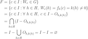
It follows from the above facts that the product space $(0,1)^\omega$ cannot be a $\sigma$ -compact space.

$\text{ }$

Proofs of Key Steps for Exercise 2.A

The proof here focuses on the example $\mathbb{R}^c$ .

To see that $W=\{W_x: x \in I \}$ has the same cardinality as that of $I$ , show that $W_x \ne W_y$ for $x \ne y$ . This follows from the definition of the mapping $W_x$ .

To see that $W$ is discrete, for each $x \in I$ , consider the open set $U_x=\{ b \in Y: b(x)=0 \}$ . Note that $W_x \in U_x$ . Further note that $W_y \notin U_x$ for all $y \ne x$ .

To see that $W$ is a closed subset of $Y$ , let $k: I \rightarrow \omega$ such that $k \notin W$ . Consider two cases.

Case 1. $k(r) \ne 0$ for all $r \in I$ .
Note that $\{ O_{t,k(t)}: t \in I \}$ is an open cover of $I$ (in the usual topology). There exists a finite $H \subset I$ such that $\{ O_{h,k(h)}: h \in H \}$ is a cover of $I$ . Consider the open set $G=\{ b \in Y: \forall \ h \in H, \ b(h)=k(h) \}$ . Define the set $F$ as follows:

$F=\{ c \in I: W_c \in G \}$

The set $F$ can be further described as follows:

$\displaystyle \begin{aligned} F&=\{ c \in I: W_c \in G \} \\&=\{ c \in I: \forall \ h \in H, \ W_c(h)=f_h(c)=k(h) \ne 0 \} \\&=\{ c \in I: \forall \ h \in H, \ c \in I-O_{h,k(h)} \} \\&=\bigcap_{h \in H} (I-O_{h,k(h)}) \\&=I-\bigcup_{h \in H} O_{h,k(h)}=I-I =\varnothing \end{aligned}$

The last step is $\varnothing$ because $\{ O_{h,k(h)}: h \in H \}$ is a cover of $I$ . The fact that $F=\varnothing$ means that $G$ is an open subset of $Y$ containing the point $k$ such that $G$ contains no point of $W$ .

Case 2. $k(r) = 0$ for some $r \in I$ .
Since $k \notin W$ , $k \ne W_x$ for all $x \in I$ . In particular, $k \ne W_r$ . This means that $k(t) \ne W_r(t)$ for some $t \in I$ . Define the open set $G$ as follows:

$G=\{ b \in Y: b(r)=0 \text{ and } b(t)=k(t) \}$

Clearly $k \in G$ . Observe that $W_r \notin G$ since $W_r(t) \ne k(t)$ . For each $p \in I-\{ r \}$ , $W_p \notin G$ since $W_p(r) \ne 0$ . Thus $G$ is an open set containing $k$ such that $G \cap W=\varnothing$ .

Both cases show that $W$ is a closed subset of $Y=\omega^I$ .

Proofs of Key Steps for Exercise 2.B

Suppose that $\mathbb{P}$ , the set of all irrational numbers, is $\sigma$ -compact. That is, $\mathbb{P}=A_1 \cup A_2 \cup A_3 \cup \cdots$ where each $A_i$ is a compact space as a subspace of $\mathbb{P}$ . Any compact subspace of $\mathbb{P}$ is also a compact subspace of $\mathbb{R}$ . As a result, each $A_i$ is a closed subset of $\mathbb{R}$ . Furthermore, prove the following:

$A_i$

$\mathbb{R}$

Each singleton set $\{ r \}$ where $r$ is any rational number is also a closed and nowhere dense subset of $\mathbb{R}$ . This means that the real line is the union of countably many closed and nowhere dense subsets, contracting the hints given earlier. Thus $\mathbb{P}$ cannot be $\sigma$ -compact.

Proofs of Key Steps for Exercise 2.C

The Sorgenfrey line $S$ is a Lindelof space whose square $S \times S$ is not normal. This is a famous example of a Lindelof space whose square is not Lindelof (not even normal). For reference, a proof is found here. An alternative proof of the non-normality of $S \times S$ uses the Baire category theorem and is found here.

If the Sorgenfrey line is $\sigma$ -compact, then $S \times S$ would be $\sigma$ -compact and hence Lindelof. Thus $S$ cannot be $\sigma$ -compact.

Proofs of Key Steps for Exercise 2.D

Suppose that $X$ is Lindelof and that $Y$ is compact. Let $\mathcal{U}$ be an open cover of $X \times Y$ . For each $x \in X$ , let $\mathcal{U}_x \subset \mathcal{U}$ be finite such that $\mathcal{U}_x$ is a cover of $\{ x \} \times Y$ . Putting it another way, $\{ x \} \times Y \subset \cup \mathcal{U}_x$ . By the Tube lemma, for each $x \in X$ , there is an open $O_x$ such that $\{ x \} \times Y \subset O_x \times Y \subset \cup \mathcal{U}_x$ . Since $X$ is Lindelof, there exists a countable set $\{ x_1,x_2,x_3,\cdots \} \subset X$ such that $\{ O_{x_1},O_{x_2},O_{x_3},\cdots \}$ is a cover of $X$ . Then $\mathcal{U}_{x_1} \cup \mathcal{U}_{x_2} \cup \mathcal{U}_{x_3} \cup \cdots$ is a countable subcover of $\mathcal{U}$ . This completes the proof that $X \times Y$ is Lindelof when $X$ is Lindelof and $Y$ is compact.

To complete the exercise, observe that if $X$ is Lindelof and $Y$ is $\sigma$ -compact, then $X \times Y$ is the union of countably many Lindelof subspaces.

Proofs of Key Steps for Exercise 2.E

Proof of Fact E.1
Let $X$ be a compact Hausdorff space. Let $O_1,O_2,O_3,\cdots$ be a sequence of non-empty open subsets of $X$ such that $latex $\overline{O_{n+1}} \subset O_n$ for each $n$ . Show that the intersection $\bigcap_{i=1}^\infty O_i$ is non-empty.

Suppose that $\bigcap_{i=1}^\infty O_i=\varnothing$ . Choose $x_1 \in O_1$ . There must exist some $n_1$ such that $x_1 \notin O_{n_1}$ . Choose $x_2 \in O_{n_1}$ . There must exist some $n_2>n_1$ such that $x_2 \notin O_{n_2}$ . Continue in this manner we can choose inductively an infinite set $A=\{ x_1,x_2,x_3,\cdots \} \subset X$ such that $x_i \ne x_j$ for $i \ne j$ . Since $X$ is compact, the infinite set $A$ has a limit point $p$ . This means that every open set containing $p$ contains some $x_j$ (in fact for infinitely many $j$ ). The point $p$ cannot be in the intersection $\bigcap_{i=1}^\infty O_i$ . Thus for some $n$ , $p \notin O_n$ . Thus $p \notin \overline{O_{n+1}}$ . We can choose an open set $U$ such that $p \in U$ and $U \cap \overline{O_{n+1}}=\varnothing$ . However, $U$ must contain some point $x_j$ where $j>n+1$ . This is a contradiction since $O_j \subset \overline{O_{n+1}}$ for all $j>n+1$ . Thus Fact E.1 is established.

Proof of Fact E.2
Let $X$ be a compact space. Let $U_1,U_2,U_3,\cdots$ be open subsets of $X$ such that each $U_i$ is also a dense subset of $X$ . Let $V$ a non-empty open subset of $X$ . We wish to show that $V$ contains a point that belongs to each $U_i$ . Since $U_1$ is dense in $X$ , $O_1=V \cap U_1$ is non-empty. Since $U_2$ is dense in $X$ , choose non-empty open $O_2$ such that $\overline{O_2} \subset O_1$ and $O_2 \subset U_2$ . Since $U_3$ is dense in $X$ , choose non-empty open $O_3$ such that $\overline{O_3} \subset O_2$ and $O_3 \subset U_3$ . Continue inductively in this manner and we have a sequence of open sets $O_1,O_2,O_3,\cdots$ just like in Fact E.1. Then the intersection of the open sets $O_n$ is non-empty. Points in the intersection are in $V$ and in all the $U_n$ . This completes the proof of Fact E.2.

Proof of Fact E.3
Let $X$ be a Baire space. Let $Y$ be a dense $G_\delta$ -subset of $X$ such that $X-Y$ is a dense subset of $X$ . Show that $Y$ is not a $\sigma$ -compact space.

Suppose $Y$ is $\sigma$ -compact. Let $Y=\bigcup_{n=1}^\infty B_n$ where each $B_n$ is compact. Each $B_n$ is obviously a closed subset of $X$ . We claim that each $B_n$ is a closed nowhere dense subset of $X$ . To see this, let $U$ be a non-empty open subset of $X$ . Since $X-Y$ is dense in $X$ , $U$ contains a point $p$ where $p \notin Y$ . Since $p \notin B_n$ , there exists a non-empty open $V \subset U$ such that $V \cap B_n=\varnothing$ . This shows that each $B_n$ is a nowhere dense subset of $X$ .

Since $Y$ is a dense $G_\delta$ -subset of $X$ , $Y=\bigcap_{n=1}^\infty O_n$ where each $O_n$ is an open and dense subset of $X$ . Then each $A_n=X-O_n$ is a closed nowhere dense subset of $X$ . This means that $X$ is the union of countably many closed and nowhere dense subsets of $X$ . More specifically, we have the following.

(1)……… $X= \biggl( \bigcup_{n=1}^\infty A_n \biggr) \cup \biggl( \bigcup_{n=1}^\infty B_n \biggr)$

Statement (1) contradicts the fact that $X$ is a Baire space. Note that all $X-A_n$ and $X-B_n$ are open and dense subsets of $X$ . Further note that the intersection of all these countably many open and dense subsets of $X$ is empty according to (1). Thus $Y$ cannot not a $\sigma$ -compact space.

Proof of Fact E.4
The space $X=[0,1]^\omega$ is compact since it is a product of compact spaces. To see that $Y=(0,1)^\omega$ is a dense $G_\delta$ -subset of $X$ , note that $Y=\bigcap_{n=1}^\infty U_n$ where for each integer $n \ge 1$

(2)……… $U_n=(0,1) \times \cdots \times (0,1) \times [0,1] \times [0,1] \times \cdots$

Note that the first $n$ factors of $U_n$ are the open interval $(0,1)$ and the remaining factors are the closed interval $[0,1]$ . It is also clear that $X-Y$ is a dense subset of $X$ . This completes the proof of Fact E.4.

$\text{ }$

Concluding Remarks

Exercise 2.A
The exercise is to show that the product of uncountably many $\sigma$ -compact spaces does not need to be Lindelof. The approach suggested in the hints is to show that $\mathbb{R}^{c}$ has uncountable extent where $c$ is continuum. Having uncountable extent (i.e. having an uncountable subset that is both closed and discrete) implies the space is not Lindelof. The uncountable extent of the product space $\mathbb{R}^{\omega_1}$ is discussed in this post.

For $\mathbb{R}^{c}$ and $\mathbb{R}^{\omega_1}$ , there is another way to show non-Lindelof. For example, both product spaces are not normal. As a result, both product spaces cannot be Lindelof. Note that every regular Lindelof space is normal. Both product spaces contain the product $\omega^{\omega_1}$ as a closed subspace. The non-normality of $\omega^{\omega_1}$ is discussed here.

Exercise 2.B
The hints given above is to show that the set of all irrational numbers, $\mathbb{P}$ , is not $\sigma$ -compact (as a subspace of the real line). The same argument showing that $\mathbb{P}$ is not $\sigma$ -compact can be generalized. Note that the complement of $\mathbb{P}$ is $\mathbb{Q}$ , the set of all rational numbers (a countable set). In this case, $\mathbb{Q}$ is a dense subset of the real line and is the union of countably many singleton sets. Each singleton set is a closed and nowhere dense subset of the real line. In general, we can let $B$ , the complement of a set $A$ , be dense in the real line and be the union of countably many closed nowhere dense subsets of the real line (not necessarily singleton sets). The same argument will show that $A$ cannot be a $\sigma$ -compact space. This argument is captured in Fact E.3 in Exercise 2.E. Thus both Exercise 2.B and Exercise 2.E use a Baire category argument.

Exercise 2.E
Like Exercise 2.B, this exercise is also to show a certain space is not $\sigma$ -compact. In this case, the suggested space is $\mathbb{R}^{\omega}$ , the product of countably many copies of the real line. The hints given use a Baire category argument, as outlined in Fact E.1 through Fact E.4. The product space $\mathbb{R}^{\omega}$ is embedded in the compact space $[0,1]^{\omega}$ , which is a Baire space. As mentioned earlier, Fact E.3 is essentially the same argument used for Exercise 2.B.

Using the same Baire category argument, it can be shown that $\omega^{\omega}$ , the product of countably many copies of the countably infinite discrete space, is not $\sigma$ -compact. The space $\omega$ of the non-negative integers, as a subspace of the real line, is certainly $\sigma$ -compact. Using the same Baire category argument, we can see that the product of countably many copies of this discrete space is not $\sigma$ -compact. With the product space $\omega^{\omega}$ , there is a connection with Exercise 2.B. The product $\omega^{\omega}$ is homeomorphic to $\mathbb{P}$ . The idea of the homeomorphism is discussed here. Thus the non- $\sigma$ -compactness of $\omega^{\omega}$ can be achieved by mapping it to the irrationals. Of course, the same Baire category argument runs through both exercises.

Exercise 2.C
Even the non- $\sigma$ -compactness of the Sorgenfrey line $S$ can be achieved by a Baire category argument. The non-normality of the Sorgenfrey plane $S \times S$ can be achieved by Jones’ lemma argument or by the fact that $\mathbb{P}$ is not a first category set. Links to both arguments are given in the Proof section above.

See here for another introduction to the Baire category theorem.

The Tube lemma is discussed here.

$\text{ }$

Dan Ma topology

Daniel Ma topology

Dan Ma math

Daniel Ma mathematics

$\copyright$ 2019 – Dan Ma

Lindelof Exercise 1

Posted on June 23, 2019 by Dan Ma

A space $X$ is called a $\sigma$ -compact space if it is the union of countably many compact subspaces. Clearly, any $\sigma$ -compact space is Lindelof. It is well known that the product of Lindelof spaces does not need to be Lindelof. The most well known example is perhaps the square of the Sorgenfrey line. In certain cases, the Lindelof property can be productive. For example, the product of countably many $\sigma$ -compact spaces is a Lindelof space. The discussion here centers on the following theorem.

Theorem 1
Let $X_1,X_2,X_3,\cdots$ be $\sigma$ -compact spaces. Then the product space $\prod_{i=1}^\infty X_i$ is Lindelof.

Theorem 1 is Exercise 3.8G in page 195 of General Topology by Engelking [1]. The reference for Exercise 3.8G is [2]. But the theorem is not found in [2] (it is not stated directly and it does not seem to be an obvious corollary of a theorem discussed in that paper). However, a hint is provided in Engelking for Exercise 3.8G. In this post, we discuss Theorem 1 as an exercise by giving expanded hint. Solutions to some of the key steps in the expanded hint are given at the end of the post.

Expanded Hint

It is helpful to first prove the following theorem.

Theorem 2
For each integer $i \ge 1$ , let $C_{i,1},C_{i,2},\cdots$ be compact spaces and let $C_i$ be the topological sum:

$C_i=C_{i,1} \oplus C_{i,2} \oplus C_{i,3} \oplus \cdots=\oplus_{j=1}^\infty C_{i,j}$

Then the product $\prod_{i=1}^\infty C_i$ is Lindelof.

Note that in the topological sum $C_{i,1} \oplus C_{i,2} \oplus C_{i,3} \oplus \cdots$ , the spaces $C_{i,1},C_{i,2},C_{i,3},\cdots$ are considered pairwise disjoint. The open sets in the sum are simply unions of the open sets in the individual spaces. Another way to view this topology: each of the $C_{i,j}$ is both closed and open in the topological sum. Theorem 2 is essentially saying that the product of countably many $\sigma$ -compact spaces is Lindelof if each $\sigma$ -compact space is the union of countably many disjoint compact spaces. The hint for Exercise 3.8G can be applied much more naturally on Theorem 2 than on Theorem 1. The following is Exercise 3.8F (a), which is the hint for Exercise 3.8G.

Lemma 3
Let $Z$ be a compact space. Let $X$ be a subspace of $Z$ . Suppose that there exist $F_1,F_2,F_3,\cdots$ , closed subsets of $Z$ , such that for all $x$ and $y$ where $x \in X$ and $y \in Z-X$ , there exists $F_i$ such that $x \in F_i$ and $y \notin F_i$ . Then $X$ is a Lindelof space.

The following theorem connects the hint (Lemma 3) with Theorem 2.

Theorem 4
For each integer $i \ge 1$ , let $Z_i$ be the one-point compactification of $C_i$ in Theorem 2. Then the product $Z=\prod_{i=1}^\infty Z_i$ is a compact space. Furthermore, $X=\prod_{i=1}^\infty C_i$ is a subspace of $Z$ . Prove that $Z$ and $X$ satisfy Lemma 3.

Each $C_i$ in Theorem 2 is a locally compact space. To define the one-point compactifications, for each $i$ , choose $p_i \notin C_i$ . Make sure that $p_i \ne p_j$ for $i \ne j$ . Then $Z_i$ is simply

$Z_i=C_i \cup \{ p_i \}=C_{i,1} \oplus C_{i,2} \oplus C_{i,3} \oplus \cdots \cup \{ p_i \}$

with the topology defined as follows:

Open subsets of $C_i$ continue to be open in $Z_i$ .
An open set containing $p_i$ is of the form $\{ p_i \} \cup (C_i - \overline{D})$ where $D$ is open in $C_i$ and $D$ is contained in the union of finitely many $C_{i,j}$ .

For convenience, each point $p_i$ is called a point at infinity.

Note that Theorem 2 follows from Lemma 3 and Theorem 4. In order to establish Theorem 1 from Theorem 2, observe that the Lindelof property is preserved by any continuous mapping and that there is a natural continuous map from the product space in Theorem 2 to the product space in Theorem 1.

$\text{ }$

Proofs of Key Steps

Proof of Lemma 3
Let $Z$ , $X$ and $F_1,F_2,F_3,\cdots$ be as described in the statement for Lemma 3. Let $\mathcal{U}$ be a collection of open subsets of $Z$ such that $\mathcal{U}$ covers $X$ . We would like to show that a countable subcollection of $\mathcal{U}$ is also a cover of $X$ . Let $O=\cup \mathcal{U}$ . If $Z-O=\varnothing$ , then $\mathcal{U}$ is an open cover of $Z$ and there is a finite subset of $\mathcal{U}$ that is a cover of $Z$ and thus a cover of $X$ . Thus we can assume that $Z-O \ne \varnothing$ .

Let $F=\{ F_1,F_2,F_3,\cdots \}$ . Let $K=Z-O$ , which is compact. We make the following claim.

Claim. Let $Y$ be the union of all possible $\cap G$ where $G \subset F$ is finite and $\cap G \subset O$ . Then $X \subset Y \subset O$ .

To establish the claim, let $x \in X$ . For each $y \in K=Z-O$ , there exists $F_{n(y)}$ such that $x \in F_{n(y)}$ and $y \notin F_{n(y)}$ . This means that $\{ Z-F_{n(y)}: y \in K \}$ is an open cover of $K$ . By the compactness of $K$ , there are finitely many $F_{n(y_1)}, \cdots, F_{n(y_k)}$ such that $F_{n(y_1)} \cap \cdots \cap F_{n(y_k)}$ misses $K$ , or equivalently $F_{n(y_1)} \cap \cdots \cap F_{n(y_k)} \subset O$ . Note that $x \in F_{n(y_1)} \cap \cdots \cap F_{n(y_k)}$ . Further note that $F_{n(y_1)} \cap \cdots \cap F_{n(y_k)} \subset Y$ . This establishes the claim that $X \subset Y$ . The claim that $Y \subset O$ is clear from the definition of $Y$ .

Each set $F_i$ is compact since it is closed in $Z$ . The intersection of finitely many $F_i$ is also compact. Thus the $\cap G$ in the definition of $Y$ in the above claim is compact. There can be only countably many $\cap G$ in the definition of $Y$ . Thus $Y$ is a $\sigma$ -compact space that is covered by the open cover $\mathcal{U}$ . Choose a countable $\mathcal{V} \subset \mathcal{U}$ such that $\mathcal{V}$ covers $Y$ . Then $\mathcal{V}$ is a cover of $X$ too. This completes the proof that $X$ is Lindelof.

$\text{ }$

Proof of Theorem 4
Recall that $Z=\prod_{i=1}^\infty Z_i$ and that $X=\prod_{i=1}^\infty C_i$ . Each $Z_i$ is the one-point compactification of $C_i$ , which is the topological sum of the disjoint compact spaces $C_{i,1},C_{i,2},\cdots$ .

For integers $i,j \ge 1$ , define $K_{i,j}=C_{i,1} \oplus C_{i,2} \oplus \cdots \oplus C_{i,j}$ . For integers $n,j \ge 1$ , define the product $F_{n,j}$ as follows:

$F_{n,j}=K_{1,j} \times \cdots \times K_{n,j} \times Z_{n+1} \times Z_{n+2} \times \cdots$

Since $F_{n,j}$ is a product of compact spaces, $F_{n,j}$ is compact and thus closed in $Z$ . There are only countably many $F_{n,j}$ .

We claim that the countably many $F_{n,j}$ have the property indicated in Lemma 3. To this end, let $f \in X=\prod_{i=1}^\infty C_i$ and $g \in Z-X$ . There exists an integer $n \ge 1$ such that $g(n) \notin C_{n}$ . This means that $g(n) \notin C_{n,j}$ for all $j$ , i.e. $g(n)=p_n$ (so $g(n)$ must be the point at infinity). Choose $j \ge 1$ large enough such that

$f(i) \in K_{i,j}=C_{i,1} \oplus C_{i,2} \oplus \cdots \oplus C_{i,j}$

for all $i \le n$ . It follows that $f \in F_{n,j}$ and $g \notin F_{n,j}$ . Thus the sequence of closed sets $F_{n,j}$ satisfies Lemma 3. By Lemma 3, $X=\prod_{i=1}^\infty C_i$ is Lindelof.

Reference

Engelking R., General Topology, Revised and Completed edition, Elsevier Science Publishers B. V., Heldermann Verlag, Berlin, 1989.
Hager A. W., Approximation of real continuous functions on Lindelof spaces, Proc. Amer. Math. Soc., 22, 156-163, 1969.

$\text{ }$

Dan Ma topology

Daniel Ma topology

Dan Ma math

Daniel Ma mathematics

$\copyright$ 2019 – Dan Ma

Every space is star discrete

Posted on October 2, 2018 by Dan Ma

The statement in the title is a folklore fact, though the term star discrete is usually not used whenever this well known fact is invoked in the literature. We present a proof to this well known fact. We also discuss some related concepts.

All spaces are assumed to be Hausdorff and regular.

First, let’s define the star notation. Let $X$ be a space. Let $\mathcal{U}$ be a collection of subsets of $X$ . Let $A \subset X$ . Define $\text{St}(A,\mathcal{U})$ to be the set $\bigcup \{U \in \mathcal{U}: U \cap A \ne \varnothing \}$ . In other words, the set $\text{St}(A,\mathcal{U})$ is simply the union of all elements of $\mathcal{U}$ that contains points of the set $A$ . The set $\text{St}(A,\mathcal{U})$ is also called the star of the set $A$ with respect to the collection $\mathcal{U}$ . If $A=\{ x \}$ , we use the notation $\text{St}(x,\mathcal{U})$ instead of $\text{St}( \{ x \},\mathcal{U})$ . The following is the well known result in question.

Lemma 1
Let $X$ be a space. For any open cover $\mathcal{U}$ of $X$ , there exists a discrete subspace $A$ of $X$ such that $X=\text{St}(A,\mathcal{U})$ . Furthermore, the set $A$ can be chosen in such a way that it is also a closed subset of the space $X$ .

Any space that satisfies the condition in Lemma 1 is said to be a star discrete space. The proof shown below will work for any topological space. Hence every space is star discrete. We come across three references in which the lemma is stated or is used – Lemma IV.2.20 in page 135 of [3], page 137 of [2] and [1]. The first two references do not use the term star discrete. Star discrete is mentioned in [1] since that paper focuses on star properties. This property that is present in every topological space is at heart a covering property. Here’s a rewording of the lemma that makes it look like a covering property.

Lemma 1a
Let $X$ be a space. For any open cover $\mathcal{U}$ of $X$ , there exists a discrete subspace $A$ of $X$ such that $\{ \text{St}(x,\mathcal{U}): x \in A \}$ is a cover of $X$ . Furthermore, the set $A$ can be chosen in such a way that it is also a closed subset of the space $X$ .

Lemma 1a is clearly identical to Lemma 1. However, Lemma 1a makes it extra clear that this is a covering property. For every open cover of a space, instead of finding a sub cover or an open refinement, we find a discrete subspace so that the stars of the points of the discrete subspace with respect to the given open cover also cover the space.

Lemma 1a naturally leads to other star covering properties. For example, a space $X$ is said to be a star countable space if for any open cover $\mathcal{U}$ of $X$ , there exists a countable subspace $A$ of $X$ such that $\{ \text{St}(x,\mathcal{U}): x \in A \}$ is a cover of $X$ . A space $X$ is said to be a star Lindelof space if for any open cover $\mathcal{U}$ of $X$ , there exists a Lindelof subspace $A$ of $X$ such that $\{ \text{St}(x,\mathcal{U}): x \in A \}$ is a cover of $X$ . In general, for any topological property $\mathcal{P}$ , a space $X$ is a star $\mathcal{P}$ space if for any open cover $\mathcal{U}$ of $X$ , there exists a subspace $A$ of $X$ with property $\mathcal{P}$ such that $\{ \text{St}(x,\mathcal{U}): x \in A \}$ is a cover of $X$ .

It follows that every Lindelof space is a star countable space. It is also clear that every star countable space is a star Lindelof space.

Lemma 1 or Lemma 1a, at first glance, may seem like a surprising result. However, one can argue that it is not a strong result at all since the property is possessed by every space. Indeed, the lemma has nothing to say about the size of the discrete set. It only says that there exists a star cover based on a discrete set for a given open cover. To derive more information about the given space, we may need to work with more information on the space in question.

Consider spaces such that every discrete subspace is countable (such a space is said to have countable spread or a space of countable spread). Also consider spaces such that every closed and discrete subspace is countable (such a space is said to have countable extent or a space of countable extent). Any space that has countable spread is also a space that has countable extent for the simple reason that if every discrete subspace is countable, then every closed and discrete subspace is countable.

Then it follows from Lemma 1 that any space $X$ that has countable extent is star countable. Any star countable space is obviously a star Lindelof space. The following diagram displays these relationships.

Countable spread and Lindelof property

According to the diagram, the star countable and star Lindelof are both downstream from the countable spread property and the Lindelof property. The star properties being downstream from the Lindelof property is not surprising. What is interesting is that if a space has countable spread, then it is star countable and hence star Lindelof.

Do “countable spread” and “Lindelof” relate to each other? Lindelof spaces do not have to have countable spread. The simplest example is the one-point compactification of an uncountable discrete space. More specifically, let $X$ be an uncountable discrete space. Let $p$ be a point not in $X$ . Then $Y=X \cup \{ p \}$ is a compact space (hence Lindelof) where $X$ is discrete and an open neighborhood of $p$ is of the form $\{ p \} \cup U$ where $X-U$ is a finite subset of $X$ . The space $Y$ is not of countable spread since $X$ is an uncountable discrete subspace.

Does “countable spread” imply “Lindelof”? Is there a non-Lindelof space that has countable spread? It turns out that the answers are independent of ZFC. The next post has more details.

We now give a proof to Lemma 1. Suppose that $X$ is an infinite space (if it is finite, the lemma is true since the space is Hausdorff). Let $\kappa=\lvert X \lvert$ . Let $\kappa^+$ be the next cardinal greater than $\kappa$ . Let $\mathcal{U}$ be an open cover of the space $X$ . Choose $x_0 \in X$ . We choose a sequence of points $x_0,x_1,\cdots,x_\alpha,\cdots$ inductively. If $\text{St}(\{x_\beta: \beta<\alpha \},\mathcal{U}) \ne X$ , we can choose a point $x_\alpha \in X$ such that $x_\alpha \notin \text{St}(\{x_\beta: \beta<\alpha \},\mathcal{U})$ .

We claim that the induction process must stop at some $\alpha<\kappa^+$ . In other words, at some $\alpha<\kappa^+$ , the star of the previous points must be the entire space and we run out of points to choose. Otherwise, we would have obtained a subset of $X$ with cardinality $\kappa^+$ , a contradiction. Choose the least $\alpha<\kappa^+$ such that $\text{St}(\{x_\beta: \beta<\alpha \},\mathcal{U}) = X$ . Let $A=\{x_\beta: \beta<\alpha \}$ .

Then it can be verified that the set $A$ is a discrete subspace of $X$ and that $A$ is a closed subset of $X$ . Note that $x_\beta \in \text{St}(x_\beta, \mathcal{U})$ while $x_\gamma \notin \text{St}(x_\beta, \mathcal{U})$ for all $\gamma \ne \beta$ . This follows from the way the points are chosen in the induction process. On the other hand, for any $x \in X-A$ , $x \in \text{St}(x_\beta, \mathcal{U})$ for some $\beta<\alpha$ . As discussed, the open set $\text{St}(x_\beta, \mathcal{U})$ contains only one point of $A$ , namely $x_\beta$ .

Reference

Alas O., Jumqueira L., van Mill J., Tkachuk V., Wilson R.On the extent of star countable spaces, Cent. Eur. J. Math., 9 (3), 603-615, 2011.
Alster, K., Pol, R.,On function spaces of compact subspaces of $\Sigma$ -products of the real line, Fund. Math., 107, 35-46, 1980.
Arkhangelskii, A. V.,Topological Function Spaces, Mathematics and Its Applications Series, Kluwer Academic Publishers, Dordrecht, 1992.

$\text{ }$

Dan Ma math

Daniel Ma mathematics

Equivalent conditions for hereditarily Lindelof spaces

Posted on May 3, 2014 by Dan Ma

A topological space $X$ is Lindelof if every open cover $X$ has a countable subcollection that also is a cover of $X$ . A topological space $X$ is hereditarily Lindelof if every subspace of $X$ , with respect to the subspace topology, is a Lindelof space. In this post, we prove a theorem that gives two equivalent conditions for the hereditarily Lindelof property. We consider the following theorem.

Theorem 1
Let $X$ be a topological space. The following conditions are equivalent.

The space $X$ is a hereditarily Lindelof space.
Every open subspace of $X$ is Lindelof.
For every uncountable subspace $Y$ of $X$ , there exists a point $y \in Y$ such that every open subset of $X$ containing $y$ contains uncountably many points of $Y$ .

This is an excellent exercise for the hereditarily Lindelof property and for transfinite induction (for one of the directions). The equivalence $1 \longleftrightarrow 3$ is the exercise 3.12.7(d) on page 224 of [1]. The equivalence of the 3 conditions of Theorem 1 is mentioned on page 182 (chapter d-8) of [2].

Proof of Theorem 1
The direction $1 \longrightarrow 2$ is immediate. The direction $2 \longrightarrow 3$ is straightforward.

$3 \longrightarrow 1$
We show $\text{not } 1 \longrightarrow \text{not } 3$ . Suppose $T$ is a non-Lindelof subspace of $X$ . Let $\mathcal{U}$ be an open cover of $T$ such that no countable subcollection of $\mathcal{U}$ can cover $T$ . By a transfinite inductive process, choose a set of points $\left\{t_\alpha \in T: \alpha < \omega_1 \right\}$ and a collection of open sets $\left\{U_\alpha \in \mathcal{U}: \alpha < \omega_1 \right\}$ such that for each $\alpha < \omega_1$ , $t_\alpha \in U_\alpha$ and $t_\alpha \notin \cup \left\{U_\beta: \beta<\alpha \right\}$ . The inductive process is possible since no countable subcollection of $\mathcal{U}$ can cover $T$ . Now let $Y=\left\{t_\alpha: \alpha<\omega_1 \right\}$ . Note that each $U_\alpha$ can at most contain countably many points of $Y$ , namely the points in $\left\{t_\beta: \beta \le \alpha \right\}$ .

For each $\alpha$ , let $V_\alpha$ be an open subset of $X$ such that $U_\alpha=V_\alpha \cap Y$ . We can now conclude: for every point $t_\alpha$ of $Y$ , there exists an open set $V_\alpha$ containing $t_\alpha$ such that $V_\alpha$ contains only countably many points of $Y$ . This is the negation of condition 3. $\blacksquare$

____________________________________________________________________

Remarks

Condition 3 indicates that every uncountable set has a certain special type of limit points. Let $p \in X$ . We say $p$ is a limit point of the set $Y \subset X$ if every open set containing $p$ contains a point of $Y$ different from $p$ . Being a limit point of $Y$ , we only know that each open set containing $p$ contain infinitely many points of $Y$ (assuming a $T_1$ space). Thus the limit points indicated in condition 3 are a special type of limit points. According to the terminology of [1], if $p$ is a limit point of $Y$ satisfying condition 3, then $p$ is said to be a condensation point of $Y$ . According to Theorem 1, existence of condensation point in every uncountable set is a strong topological property (being equivalent to the hereditarily property). It is easy to see that of condition 3 holds, all but countably many points of any uncountable set $Y$ is a condensation point of $Y$ .

In some situations, we may not need the full strength of condition 3. In such situations, the following corollary may be sufficient.

Corollary 2
If the space $X$ is hereditarily Lindelof, then every uncountable subspace $Y$ of $X$ contains one of its limit points.

As noted earlier, if every uncountable set contains one of its limits, then all but countably many points of any uncountable set are limit points. To contrast the hereditarily Lindelof property with the Lindelof property, consider the following theorem.

Theorem 3
If the space $X$ is Lindelof, then every uncountable subspace $Y$ of $X$ has a limit point.

The condition “every uncountable subspace $Y$ of $X$ has a limit point” has another name. When a space satisfies this condition, it is said to have countable extent. The ideas in Corollary 2 and Theorem 3 are also discussed in this previous post.

____________________________________________________________________

Reference

Engelking, R., General Topology, Revised and Completed edition, Heldermann Verlag, Berlin, 1989.
Hart, K. P., Nagata J. I., Vaughan, J. E., editors, Encyclopedia of General Topology, First Edition, Elsevier Science Publishers B. V, Amsterdam, 2003.

____________________________________________________________________

An example of a normal but not Lindelof Cp(X)

Posted on May 1, 2014 by Dan Ma

In this post, we discuss an example of a function space $C_p(X)$ that is normal and not Lindelof (as indicated in the title). Interestingly, much more can be said about this function space. In this post, we show that there exists a space $X$ such that

$C_p(X)$ is collectionwise normal and not paracompact,
$C_p(X)$ is not Lindelof but contains a dense Lindelof subspace,
$C_p(X)$ is not first countable but is a Frechet space,
As a corollary of the previous point, $C_p(X)$ cannot contain a copy of the compact space $\omega_1+1$ ,
$C_p(X)$ is homeomorphic to $C_p(X)^\omega$ ,
$C_p(X)$ is not hereditarily normal,
$C_p(X)$ is not metacompact.

A short and quick description of the space $X$ is that $X$ is the one-point Lindelofication of an uncountable discrete space. As shown below, the function space $C_p(X)$ is intimately related to a $\Sigma$ -product of copies of real lines. The results listed above are merely an introduction to this wonderful example and are derived by examining the $\Sigma$ -products of copies of real lines. Deep results about $\Sigma$ -product of real lines abound in the literature. The references listed at the end are a small sample. Example 3.2 in [2] is another interesting illustration of this example.

We now define the domain space $X=L_\tau$ . In the discussion that follows, the Greek letter $\tau$ is always an uncountable cardinal number. Let $D_\tau$ be a set with cardinality $\tau$ . Let $p$ be a point not in $D_\tau$ . Let $L_\tau=D_\tau \cup \left\{p \right\}$ . Consider the following topology on $L_\tau$ :

Each point in $D_\tau$ an isolated point, and
open neighborhoods at the point $p$ are of the form $L_\tau-K$ where $K \subset D_\tau$ is countable.

It is clear that $L_\tau$ is a Lindelof space. The Lindelof space $L_\tau$ is sometimes called the one-point Lindelofication of the discrete space $D_\tau$ since it is a Lindelof space that is obtained by adding one point to a discrete space.

Consider the function space $C_p(L_\tau)$ . See this post for general information on the pointwise convergence topology of $C_p(Y)$ for any completely regular space $Y$ .

All the facts about $C_p(X)=C_p(L_\tau)$ mentioned at the beginning follow from the fact that $C_p(L_\tau)$ is homeomorphic to the $\Sigma$ -product of $\tau$ many copies of the real lines. Specifically, $C_p(L_\tau)$ is homeomorphic to the following subspace of the product space $\mathbb{R}^\tau$ .

$\Sigma_{\alpha<\tau}\mathbb{R}=\left\{ x \in \mathbb{R}^\tau: x_\alpha \ne 0 \text{ for at most countably many } \alpha<\tau \right\}$

Thus understanding the function space $C_p(L_\tau)$ is a matter of understanding a $\Sigma$ -product of copies of the real lines. First, we establish the homeomorphism and then discuss the properties of $C_p(L_\tau)$ indicated above.

____________________________________________________________________

The Homeomorphism

For each $f \in C_p(L_\tau)$ , it is easily seen that there is a countable set $C \subset D_\tau$ such that $f(p)=f(y)$ for all $y \in D_\tau-C$ . Let $W_0=\left\{f \in C_p(L_\tau): f(p)=0 \right\}$ . Then each $f \in W_0$ has non-zero values only on a countable subset of $D_\tau$ . Naturally, $W_0$ and $\Sigma_{\alpha<\tau}\mathbb{R}$ are homeomorphic.

We claim that $C_p(L_\tau)$ is homeomorphic to $W_0 \times \mathbb{R}$ . For each $f \in C_p(L_\tau)$ , define $h(f)=(f-f(p),f(p))$ . Here, $f-f(p)$ is the function $g \in C_p(L_\tau)$ such that $g(x)=f(x)-f(p)$ for all $x \in L_\tau$ . Clearly $h(f)$ is well-defined and $h(f) \in W_0 \times \mathbb{R}$ . It can be readily verified that $h$ is a one-to-one map from $C_p(L_\tau)$ onto $W_0 \times \mathbb{R}$ . It is not difficult to verify that both $h$ and $h^{-1}$ are continuous.

We use the notation $X_1 \cong X_2$ to mean that the spaces $X_1$ and $X_2$ are homeomorphic. Then we have:

$C_p(L_\tau) \ \cong \ W_0 \times \mathbb{R} \ \cong \ (\Sigma_{\alpha<\tau}\mathbb{R}) \times \mathbb{R} \ \cong \ \Sigma_{\alpha<\tau}\mathbb{R}$

Thus $C_p(L_\tau) \ \cong \ \Sigma_{\alpha<\tau}\mathbb{R}$ . This completes the proof that $C_p(L_\tau)$ is topologically the $\Sigma$ -product of $\tau$ many copies of the real lines.

____________________________________________________________________

Looking at the $\Sigma$ -Product

Understanding the function space $C_p(L_\tau)$ is now reduced to the problem of understanding a $\Sigma$ -product of copies of the real lines. Most of the facts about $\Sigma$ -products that we need have already been proved in previous blog posts.

In this previous post, it is established that the $\Sigma$ -product of separable metric spaces is collectionwise normal. Thus $C_p(L_\tau)$ is collectionwise normal. The $\Sigma$ -product of spaces, each of which has at least two points, always contains a closed copy of $\omega_1$ with the ordered topology (see the lemma in this previous post). Thus $C_p(L_\tau)$ contains a closed copy of $\omega_1$ and hence can never be paracompact (and thus not Lindelof).

___________________________________

Consider the following subspace of the $\Sigma$ -product $\Sigma_{\alpha<\tau}\mathbb{R}$ :

$\sigma_\tau=\left\{ x \in \Sigma_{\alpha<\tau}\mathbb{R}: x_\alpha \ne 0 \text{ for at most finitely many } \alpha<\tau \right\}$

In this previous post, it is shown that $\sigma_\tau$ is a Lindelof space. Though $C_p(L_\tau) \cong \Sigma_{\alpha<\tau}\mathbb{R}$ is not Lindelof, it has a dense Lindelof subspace, namely $\sigma_\tau$ .

___________________________________

A space $Y$ is first countable if there exists a countable local base at each point $y \in Y$ . A space $Y$ is a Frechet space (or is Frechet-Urysohn) if for each $y \in Y$ , if $y \in \overline{A}$ where $A \subset Y$ , then there exists a sequence $\left\{y_n: n=1,2,3,\cdots \right\}$ of points of $A$ such that the sequence converges to $y$ . Clearly, any first countable space is a Frechet space. The converse is not true (see Example 1 in this previous post).

For any uncountable cardinal number $\tau$ , the product $\mathbb{R}^\tau$ is not first countable. In fact, any dense subspace of $\mathbb{R}^\tau$ is not first countable. In particular, the $\Sigma$ -product $\Sigma_{\alpha<\tau}\mathbb{R}$ is not first countable. In this previous post, it is shown that the $\Sigma$ -product of first countable spaces is a Frechet space. Thus $C_p(L_\tau) \cong \Sigma_{\alpha<\tau}\mathbb{R}$ is a Frechet space.

___________________________________

As a corollary of the previous point, $C_p(L_\tau) \cong \Sigma_{\alpha<\tau}\mathbb{R}$ cannot contain a homeomorphic copy of any space that is not Frechet. In particular, it cannot contain a copy of any compact space that is not Frechet. For example, the compact space $\omega_1+1$ is not embeddable in $C_p(L_\tau)$ . The interest in compact subspaces of $C_p(L_\tau) \cong \Sigma_{\alpha<\tau}\mathbb{R}$ is that any compact space that is topologically embeddable in a $\Sigma$ -product of real lines is said to be Corson compact. Thus any Corson compact space is a Frechet space.

___________________________________

It can be readily verified that

$\Sigma_{\alpha<\tau}\mathbb{R} \ \cong \ \Sigma_{\alpha<\tau}\mathbb{R} \ \times \ \Sigma_{\alpha<\tau}\mathbb{R} \ \times \ \Sigma_{\alpha<\tau}\mathbb{R} \ \times \ \cdots \ \text{(countably many times)}$

Thus $C_p(L_\tau) \cong C_p(L_\tau)^\omega$ . In particular, $C_p(L_\tau) \cong C_p(L_\tau) \times C_p(L_\tau)$ due to the following observation:

$C_p(L_\tau) \times C_p(L_\tau) \cong C_p(L_\tau)^\omega \times C_p(L_\tau)^\omega \cong C_p(L_\tau)^\omega \cong C_p(L_\tau)$

___________________________________

As a result of the peculiar fact that $C_p(L_\tau) \cong C_p(L_\tau) \times C_p(L_\tau)$ , it can be concluded that $C_p(L_\tau)$ , though normal, is not hereditarily normal. This follows from an application of Katetov’s theorem. The theorem states that if $Y_1 \times Y_2$ is hereditarily normal, then either $Y_1$ is perfectly normal or every countably infinite subset of $Y_2$ is closed and discrete (see this previous post). The function space $C_p(L _\tau)$ is not perfectly normal since it contains a closed copy of $\omega_1$ . On the other hand, there are plenty of countably infinite subsets of $C_p(L _\tau)$ that are not closed and discrete. As a Frechet space, $C_p(L _\tau)$ has many convergent sequences. Each such sequence without the limit is a countably infinite set that is not closed and discrete. As an example, let $\left\{x_1,x_2,x_3,\cdots \right\}$ be an infinite subset of $D_\tau$ and consider the following:

$C=\left\{f_n: n=1,2,3,\cdots \right\}$

where $f_n$ is such that $f_n(x_n)=n$ and $f_n(x)=0$ for each $x \in L_\tau$ with $x \ne x_n$ . Note that $C$ is not closed and not discrete since the points in $C$ converge to $g \in \overline{C}$ where $g$ is the zero-function. Thus $C_p(L_\tau) \cong C_p(L_\tau) \times C_p(L_\tau)$ is not hereditarily normal.

___________________________________

It is well known that collectionwise normal metacompact space is paracompact (see Theorem 5.3.3 in [4] where metacompact is referred to as weakly paracompact). Since $C_p(L_\tau)$ is collectionwise normal and not paracompact, $C_p(L_\tau)$ can never be metacompact.

____________________________________________________________________

Reference

Arkhangelskii, A. V., Topological Function Spaces, Mathematics and Its Applications Series, Kluwer Academic Publishers, Dordrecht, 1992.
Bella, A., Masami, S., Tight points of Pixley-Roy hyperspaces, Topology Appl., 160, 2061-2068, 2013.
Corson, H. H., Normality in subsets of product spaces, Amer. J. Math., 81, 785-796, 1959.
Engelking, R., General Topology, Revised and Completed edition, Heldermann Verlag, Berlin, 1989.

____________________________________________________________________

(Lower case) sigma-products of separable metric spaces are Lindelof

Posted on April 21, 2014 by Dan Ma

Consider the product space $X=\prod_{\alpha \in A} X_\alpha$ . Fix a point $b \in \prod_{\alpha \in A} X_\alpha$ , called the base point. The $\Sigma$ -product of the spaces $\left\{X_\alpha: \alpha \in A \right\}$ is the following subspace of the product space $X$ :

$\Sigma_{\alpha \in A} X_\alpha=\left\{ x \in X: x_\alpha \ne b_\alpha \text{ for at most countably many } \alpha \in A \right\}$

In other words, the space $\Sigma_{\alpha \in A} X_\alpha$ is the subspace of the product space $X=\prod_{\alpha \in A} X_\alpha$ consisting of all points that deviate from the base point on at most countably many coordinates $\alpha \in A$ . We also consider the following subspace of $\Sigma_{\alpha \in A} X_\alpha$ .

$\sigma=\left\{ x \in \Sigma_{\alpha \in A} X_\alpha: x_\alpha \ne b_\alpha \text{ for at most finitely many } \alpha \in A \right\}$

For convenience , we call $\Sigma_{\alpha \in A} X_\alpha$ the (upper case) Sigma-product (or $\Sigma$ -product) of the spaces $X_\alpha$ and we call the space $\sigma$ the (lower case) sigma-product (or $\sigma$ -product). Clearly, the space $\sigma$ is a dense subspace of $\Sigma_{\alpha \in A} X_\alpha$ . In a previous post, we show that the upper case Sigma-product of separable metric spaces is collectionwise normal. In this post, we show that the (lower case) sigma-product of separable metric spaces is Lindelof. Thus when each factor $X_\alpha$ is a separable metric space with at least two points, the $\Sigma$ -product, though not Lindelof, has a dense Lindelof subspace. The (upper case) $\Sigma$ -product of separable metric spaces is a handy example of a non-Lindelof space that contains a dense Lindelof subspace.

Naturally, the lower case sigma-product can be further broken down into countably many subspaces. For each integer $n=0,1,2,3,\cdots$ , we define $\sigma_n$ as follows:

$\sigma_n=\left\{ x \in \sigma: x_\alpha \ne b_\alpha \text{ for at most } n \text{ many } \alpha \in A \right\}$

Clearly, $\sigma=\bigcup_{n=0}^\infty \sigma_n$ . We prove the following theorem. The fact that $\sigma$ is Lindelof will follow as a corollary. Understanding the following proof for Theorem 1 is a matter of keeping straight the notations involving standard basic open sets in the product space $X=\prod_{\alpha \in A} X_\alpha$ . We say $V$ is a standard basic open subset of the product space $X$ if $V$ is of the form $V=\prod_{\alpha \in A} V_\alpha$ such that each $V_\alpha$ is an open subset of the factor space $X_\alpha$ and $V_\alpha=X_\alpha$ for all but finitely many $\alpha \in A$ . The finite set $F$ of all $\alpha \in A$ such that $V_\alpha \ne X_\alpha$ is called the support of the open set $V$ .

Theorem 1
Let $\sigma$ be the $\sigma$ -product of the separable metrizable spaces $\left\{X_\alpha: \alpha \in A \right\}$ . For each $n$ , let $\sigma_n$ be defined as above. The product space $\sigma_n \times Y$ is Lindelof for each non-negative integer $n$ and for all separable metric space $Y$ .

Proof of Theorem 1
We prove by induction on $n$ . Note that $\sigma_0=\left\{b \right\}$ , the base point. Clearly $\sigma_0 \times Y$ is Lindelof for all separable metric space $Y$ . Suppose the theorem hold for the integer $n$ . We show that $\sigma_{n+1} \times Y$ for all separable metric space $Y$ . To this end, let $\mathcal{U}$ be an open cover of $\sigma_{n+1} \times Y$ where $Y$ is a separable metric space. Without loss of generality, we assume that each element of $\mathcal{U}$ is of the form $V \times W$ where $V=\prod_{\alpha \in A} V_\alpha$ is a standard basic open subset of the product space $X=\prod_{\alpha \in A} X_\alpha$ and $W$ is an open subset of $Y$ .

Let $\mathcal{U}_0=\left\{U_1,U_2,U_3,\cdots \right\}$ be a countable subcollection of $\mathcal{U}$ such that $\mathcal{U}_0$ covers $\left\{b \right\} \times Y$ . For each $j$ , let $U_j=V_j \times W_j$ where $V_j=\prod_{\alpha \in A} V_{j,\alpha}$ is a standard basic open subset of the product space $X$ with $b \in V_j$ and $W_j$ is an open subset of $Y$ . For each $j$ , let $F_j$ be the support of $V_j$ . Note that $\alpha \in F_j$ if and only if $V_{j,\alpha} \ne X_\alpha$ . Also for each $\alpha \in F_j$ , $b_\alpha \in V_{j,\alpha}$ . Furthermore, for each $\alpha \in F_j$ , let $V^c_{j,\alpha}=X_\alpha- V_{j,\alpha}$ . With all these notations in mind, we define the following open set for each $\beta \in F_j$ :

$H_{j,\beta}= \biggl( V^c_{j,\beta} \times \prod_{\alpha \in A, \alpha \ne \beta} X_\alpha \biggr) \times W_j=\biggl( V^c_{j,\beta} \times T_\beta \biggr) \times W_j$

Observe that for each point $y \in \sigma_{n+1}$ such that $y \in V^c_{j,\beta} \times T_\beta$ , the point $y$ already deviates from the base point $b$ on one coordinate, namely $\beta$ . Thus on the coordinates other than $\beta$ , the point $y$ can only deviates from $b$ on at most $n$ many coordinates. Thus $\sigma_{n+1} \cap (V^c_{j,\beta} \times T_\beta)$ is homeomorphic to $V^c_{j,\beta} \times \sigma_n$ . Note that $V^c_{j,\beta} \times W_j$ is a separable metric space. By inductive hypothesis, $V^c_{j,\beta} \times \sigma_n \times W_j$ is Lindelof. Thus there are countably many open sets in the open cover $\mathcal{U}$ that covers points of $H_{j,\beta} \cap (\sigma_{n+1} \times W_j)$ .

Note that

$\sigma_{n+1} \times Y=\biggl( \bigcup_{j=1}^\infty U_j \cap \sigma_{n+1} \biggr) \cup \biggl( \bigcup \left\{H_{j,\beta} \cap (\sigma_{n+1} \times W_j): j=1,2,3,\cdots, \beta \in F_j \right\} \biggr)$

To see that the left-side is a subset of the right-side, let $t=(x,y) \in \sigma_{n+1} \times Y$ . If $t \in U_j$ for some $j$ , we are done. Suppose $t \notin U_j$ for all $j$ . Observe that $y \in W_j$ for some $j$ . Since $t=(x,y) \notin U_j$ , $x_\beta \notin V_{j,\beta}$ for some $\beta \in F_j$ . Then $t=(x,y) \in H_{j,\beta}$ . It is now clear that $t=(x,y) \in H_{j,\beta} \cap (\sigma_{n+1} \times W_j)$ . Thus the above set equality is established. Thus one part of $\sigma_{n+1} \times Y$ is covered by countably many open sets in $\mathcal{U}$ while the other part is the union of countably many Lindelof subspaces. It follows that a countable subcollection of $\mathcal{U}$ covers $\sigma_{n+1} \times Y$ . $\blacksquare$

Corollary 2
It follows from Theorem 1 that

If each factor space $X_\alpha$ is a separable metric space, then each $\sigma_n$ is a Lindelof space and that $\sigma=\bigcup_{n=0}^\infty \sigma_n$ is a Lindelof space.
If each factor space $X_\alpha$ is a compact separable metric space, then each $\sigma_n$ is a compact space and that $\sigma=\bigcup_{n=0}^\infty \sigma_n$ is a $\sigma$ -compact space.

Proof of Corollary 2
The first bullet point is a clear corollary of Theorem 1. A previous post shows that $\Sigma$ -product of compact spaces is countably compact. Thus $\Sigma_{\alpha \in A} X_\alpha$ is a countably compact space if each $X_\alpha$ is compact. Note that each $\sigma_n$ is a closed subset of $\Sigma_{\alpha \in A} X_\alpha$ and is thus countably compact. Being a Lindelof space, each $\sigma_n$ is compact. It follows that $\sigma=\bigcup_{n=0}^\infty \sigma_n$ is a $\sigma$ -compact space. $\blacksquare$

____________________________________________________________________

A non-Lindelof space with a dense Lindelof subspace

Now we put everything together to obtain the example described at the beginning. For each $\alpha \in A$ , let $X_\alpha$ be a separable metric space with at least two points. Then the $\Sigma$ -product $\Sigma_{\alpha \in A} X_\alpha$ is collectionwise normal (see this previous post). According to the lemma in this previous post, the $\Sigma$ -product $\Sigma_{\alpha \in A} X_\alpha$ contains a closed copy of $\omega_1$ . Thus the $\Sigma$ -product $\Sigma_{\alpha \in A} X_\alpha$ is not Lindelof. It is clear that the $\sigma$ -product is a dense subspace of $\Sigma_{\alpha \in A} X_\alpha$ . By Corollary 2, the $\sigma$ -product is a Lindelof subspace of $\Sigma_{\alpha \in A} X_\alpha$ .

Using specific factor spaces, if each $X_\alpha=\mathbb{R}$ with the usual topology, then $\Sigma_{\alpha<\omega_1} X_\alpha$ is a non-Lindelof space with a dense Lindelof subspace. On the other hand, if each $X_\alpha=[0,1]$ with the usual topology, then $\Sigma_{\alpha<\omega_1} X_\alpha$ is a non-Lindelof space with a dense $\sigma$ -compact subspace. Another example of a non-Lindelof space with a dense Lindelof subspace is given In this previous post (see Example 1).

____________________________________________________________________

Cp(X) where X is a separable metric space

Posted on April 3, 2014 by Dan Ma

Let $\tau$ be an uncountable cardinal. Let $\prod_{\alpha < \tau} \mathbb{R}=\mathbb{R}^{\tau}$ be the Cartesian product of $\tau$ many copies of the real line. This product space is not normal since it contains $\prod_{\alpha \in \omega_1} \omega=\omega^{\omega_1}$ as a closed subspace. However, there are dense subspaces of $\mathbb{R}^{\tau}$ are normal. For example, the $\Sigma$ -product of $\tau$ copies of the real line is normal, i.e., the subspace of $\mathbb{R}^{\tau}$ consisting of points which have at most countably many non-zero coordinates (see this post). In this post, we look for more normal spaces among the subspaces of $\mathbb{R}^{\tau}$ that are function spaces. In particular, we look at spaces of continuous real-valued functions defined on a separable metrizable space, i.e., the function space $C_p(X)$ where $X$ is a separable metrizable space.

For definitions of basic open sets and other background information on the function space $C_p(X)$ , see this previous post.

____________________________________________________________________

$C_p(X)$ when $X$ is a separable metric space

In the remainder of the post, $X$ denotes a separable metrizable space. Then, $C_p(X)$ is more than normal. The function space $C_p(X)$ has the following properties:

normal,
Lindelof (hence paracompact and collectionwise normal),
hereditarily Lindelof (hence hereditarily normal),
hereditarily separable,
perfectly normal.

All such properties stem from the fact that $C_p(X)$ has a countable network whenever $X$ is a separable metrizable space.

Let $L$ be a topological space. A collection $\mathcal{N}$ of subsets of $L$ is said to be a network for $L$ if for each $x \in L$ and for each open $O \subset L$ with $x \in O$ , there exists some $A \in \mathcal{N}$ such that $x \in A \subset O$ . A countable network is a network that has only countably many elements. The property of having a countable network is a very strong property, e.g., having all the properties listed above. For a basic discussion of this property, see this previous post and this previous post.

To define a countable network for $C_p(X)$ , let $\mathcal{B}$ be a countable base for the domain space $X$ . For each $B \subset \mathcal{B}$ and for any open interval $(a,b)$ in the real line with rational endpoints, consider the following set:

$[B,(a,b)]=\left\{f \in C(X): f(B) \subset (a,b) \right\}$

There are only countably many sets of the form $[B,(a,b)]$ . Let $\mathcal{N}$ be the collection of sets, each of which is the intersection of finitely many sets of the form $[B,(a,b)]$ . Then $\mathcal{N}$ is a network for the function space $C_p(X)$ . To see this, let $f \in O$ where $O=\bigcap_{x \in F} [x,O_x]$ is a basic open set in $C_p(X)$ where $F \subset X$ is finite and each $O_x$ is an open interval with rational endpoints. For each point $x \in F$ , choose $B_x \in \mathcal{B}$ with $x \in B_x$ such that $f(B_x) \subset O_x$ . Clearly $f \in \bigcap_{x \in F} \ [B_x,O_x]$ . It follows that $\bigcap_{x \in F} \ [B_x,O_x] \subset O$ .

Examples include $C_p(\mathbb{R})$ , $C_p([0,1])$ and $C_p(\mathbb{R}^\omega)$ . All three can be considered subspaces of the product space $\mathbb{R}^c$ where $c$ is the cardinality of the continuum. This is true for any separable metrizable $X$ . Note that any separable metrizable $X$ can be embedded in the product space $\mathbb{R}^\omega$ . The product space $\mathbb{R}^\omega$ has cardinality $c$ . Thus the cardinality of any separable metrizable space $X$ is at most continuum. So $C_p(X)$ is the subspace of a product space of $\le$ continuum many copies of the real lines, hence can be regarded as a subspace of $\mathbb{R}^c$ .

A space $L$ has countable extent if every closed and discrete subset of $L$ is countable. The $\Sigma$ -product $\Sigma_{\alpha \in A} X_\alpha$ of the separable metric spaces $\left\{X_\alpha: \alpha \in A \right\}$ is a dense and normal subspace of the product space $\prod_{\alpha \in A} X_\alpha$ . The normal space $\Sigma_{\alpha \in A} X_\alpha$ has countable extent (hence collectionwise normal). The examples of $C_p(X)$ discussed here are Lindelof and hence have countable extent. Many, though not all, dense normal subspaces of products of separable metric spaces have countable extent. For a dense normal subspace of a product of separable metric spaces, one interesting problem is to find out whether it has countable extent.

____________________________________________________________________

Dan Ma's Topology Blog

Expository Articles In General Topology

Tag Archives: Lindelof space

Perfect preimages of Lindelof spaces

A Pixley-Roy Meta-Lindelof Space

Examples of Meta-Lindelof Spaces

Lindelof Exercise 2

Lindelof Exercise 1

Every space is star discrete

Equivalent conditions for hereditarily Lindelof spaces

An example of a normal but not Lindelof Cp(X)

(Lower case) sigma-products of separable metric spaces are Lindelof

Cp(X) where X is a separable metric space