September | 2017 | Dan Ma's Topology Blog

The Sorgenfrey line is a well known topological space. It is the real number line with open intervals defined as sets of the form $[a,b)$ . Though this is a seemingly small tweak, it generates a vastly different space than the usual real number line. In this post, we look at the Sorgenfrey line from the continuous function perspective, in particular, the continuous functions that map the Sorgenfrey line into the real number line. In the process, we obtain insight into the space of continuous functions on the Sorgenfrey line.

The next post is a continuation on the theme of drawing Sorgenfrey continuous functions.

The Sorgenfrey Line

Let $\mathbb{R}$ denote the real number line. The usual open intervals are of the form $(a,b)=\left\{x \in \mathbb{R}: a<x<b \right\}$ . The union of such open intervals is called an open set. If more than one topologies are considered on the real line, these open sets are referred to as the usual open sets or Euclidean open sets (on the real line). The open intervals $(a,b)$ form a base for the usual topology on the real line. One important fact abut the usual open sets is that the usual open sets can be generated by the intervals $(a,b)$ where both end points are rational numbers. Thus the usual topology on the real line is said to have a countable base.

Now tweak the usual topology by calling sets of the form $[a,b)=\left\{x \in \mathbb{R}: a \le x<b \right\}$ open intervals. Then form open sets by taking unions of all such open intervals. The collection of such open sets is called the Sorgenfrey topology (on the real line). The real number line $\mathbb{R}$ with the Sorgenfry topology is called the Sorgenfrey line, denoted by $\mathbb{S}$ . The Sorgenfrey line has been discussed in this blog, starting with this post. This post examines continuous functions from $\mathbb{S}$ into the real line. In the process, we gain insight on the space of continuous functions defined on $\mathbb{S}$ .

Note that any usual open interval $(a,b)$ is the union of intervals of the form $[c,d)$ . Thus any usual (Euclidean) open set is an open set in the Sorgenfrey line. Thus the usual topology (on the real line) is contained in the Sorgenfrey topology, i.e. the usual topology is a weaker (coarser) topology.

Let $C(\mathbb{R})$ be the set of all continuous functions $f:\mathbb{R} \rightarrow \mathbb{R}$ where the domain is the real number line with the usual topology. Let $C(\mathbb{S})$ be the set of all continuous functions $f:\mathbb{S} \rightarrow \mathbb{R}$ where the domain is the Sorgenfrey line. In both cases, the range is always the number line with the usual topology. Based on the preceding paragraph, any continuous function $f:\mathbb{R} \rightarrow \mathbb{R}$ is also continuous with respect to the Sorgenfrey line, i.e. $C(\mathbb{R}) \subset C(\mathbb{S})$ .

Pictures of Continuous Functions

Consider the following two continuous functions.

Figure 1 – CDF of the standard normal distribution

Figure 2 – CDF of the uniform distribution

The first one (Figure 1) is the cumulative distribution function (CDF) of the standard normal distribution. The second one (Figure 2) is the CDF of the uniform distribution on the interval $(0,a)$ where $a>0$ . Both of these are continuous in the usual Euclidean topology (in the domain). Such graphs would make regular appearance in a course on probability and statistics. They also show up in a calculus course as an everywhere differentiable curve (Figure 1) and as a differentiable curve except at finitely many points (Figure 2). Both of these functions can also be regarded as continuous functions on the Sorgenfrey line.

Consider a function that is continuous in the Sorgenfrey line but not continuous in the usual topology.

Figure 3 – Right continuous function

Figure 3 is a function that maps the interval $(-\infty,0)$ to -1 and maps the interval $[0,\infty)$ to 1. It is not continuous in the usual topology because of the jump at $x=0$ . But it is a continuous function when the domain is considered to be the Sorgenfrey line. Because of the open intervals being $[a,b)$ , continuous functions defined on the Sorgenfrey line are right continuous.

The cumulative distribution function of a discrete probability distribution is always right continuous, hence continuous in the Sorgenfrey line. Here’s an example.

Figure 4 – CDF of a discrete uniform distribution

Figure 4 is the CDF of the uniform distribution on the finite set $\left\{0,1,2,3,4 \right\}$ , where each point has probability 0.2. There is a jump of height 0.2 at each of the points from 0 to 4. Figure 3 and Figure 4 are step functions. As long as the left point of a step is solid and the right point is hollow, the step functions are continuous on the Sorgenfrey line.

The take away from the last four figures is that the real-valued continuous functions defined on the Sorgenfrey line are right continuous and that step functions (with the left point solid and the right point hollow) are Sorgenfrey continuous.

A Family of Sorgenfrey Continuous Functions

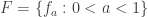
The four examples of continuous functions shown above are excellent examples to illustrate the Sorgenfrey topology. We now introduce a family of continuous functions $f_a:\mathbb{S} \rightarrow \mathbb{R}$ for $0<a<1$ . These continuous functions will lead to additional insight on the function space whose domain space is the Sorgenfrey line.

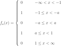
For any $0<a<1$ , the following gives the definition and the graph of the function $f_a$ .

$\displaystyle f_a(x) = \left\{ \begin{array}{ll} \displaystyle 0 &\ \ \ \ \ \ -\infty<x<-1 \\ \text{ } & \text{ } \\ \displaystyle 1 &\ \ \ \ \ \ -1 \le x<-a \\ \text{ } & \text{ } \\ 0 &\ \ \ \ \ \ -a \le x <a \\ \text{ } & \text{ } \\ 1 &\ \ \ \ \ \ a \le x <1 \\ \text{ } & \text{ } \\ 0 &\ \ \ \ \ \ 1 \le x <\infty \end{array} \right.$

Figure 5 – a family of Sorgenfrey continuous functions

Function Space on the Sorgenfrey Line

This is the place where we switch the focus to function space. The set $C(\mathbb{S})$ is a subset of the product space $\mathbb{R}^\mathbb{R}$ . So we can consider $C(\mathbb{S})$ as a topological space endowed with the topology inherited as a subspace of $\mathbb{R}^\mathbb{R}$ . This topology on $C(\mathbb{S})$ is called the pointwise convergence topology and $C(\mathbb{S})$ with the product subspace topology is denoted by $C_p(\mathbb{S})$ . See here for comments on how to work with the pointwise convergence topology.

For the present discussion, all we need is some notation on a base for $C_p(\mathbb{S})$ . For $x \in \mathbb{S}$ , and for any open interval $(a,b)$ (open in the usual topology of the real number line), let $[x,(a,b)]=\left\{h \in C_p(\mathbb{S}): h(x) \in (a, b) \right\}$ . Then the collection of intersections of finitely many $[x,(a,b)]$ would form a base for $C_p(\mathbb{S})$ .

The following is the main fact we wish to establish.

The function space $C_p(\mathbb{S})$ contains a closed and discrete subspace of cardinality continuum. In particular, the set $F=\left\{f_a: 0<a<1 \right\}$ is a closed and discrete subspace of $C_p(\mathbb{S})$ .

The above result will derive several facts on the function space $C_p(\mathbb{S})$ , which are discussed in a section below. More interestingly, the proof of the fact that $F=\left\{f_a: 0<a<1 \right\}$ is a closed and discrete subspace of $C_p(\mathbb{S})$ is based purely on the definition of the functions $f_a$ and the Sorgenfrey topology. The proof given below does not use any deep or high powered results from function space theory. So it should be a nice exercise on the Sorgenfrey topology.

I invite readers to either verify the fact independently of the proof given here or follow the proof closely. Lots of drawing of the functions $f_a$ on paper will be helpful in going over the proof. In this one instance at least, drawing continuous functions can help gain insight on function spaces.

Working out the Proof

The following diagram was helpful to me as I worked out the different cases in showing the discreteness of the family $F=\left\{f_a: 0<a<1 \right\}$ . The diagram is a valuable aid in convincing myself that a given case is correct.

Figure 6 – A comparison of three Sorgenfrey continuous functions

Now the proof. First, $F$ is relatively discrete in $C_p(\mathbb{S})$ . We show that for each $a$ , there is an open set $O$ containing $f_a$ such that $O$ does not contain $f_w$ for any $w \ne a$ . To this end, let $O=[a,V_1] \cap [-a,V_2]$ where $V_1$ and $V_2$ are the open intervals $V_1=(0.9,1.1)$ and $V_2=(-0.1,0.1)$ . With Figure 6 as an aid, it follows that for $0<b<a$ , $f_b \notin O$ and for $a<c<1$ , $f_c \notin O$ .

The open set $O=[a,V_1] \cap [-a,V_2]$ contains $f_a$ , the function in the middle of Figure 6. Note that for $0<b<a$ , $f_b(-a)=1$ and $f_b(-a) \notin V_2$ . Thus $f_b \notin O$ . On the other hand, for $a<c<1$ , $f_c(a)=0$ and $f_c(a) \notin V_1$ . Thus $f_c \notin O$ . This proves that the set $F$ is a discrete subspace of $C_p(\mathbb{S})$ relative to $F$ itself.

Now we show that $F$ is closed in $C_p(\mathbb{S})$ . To this end, we show that

$g \in C_p(\mathbb{S})$

$U$

$g$

$U$

$F$

Actually, this has already been done above with points $g$ that are in $F$ . One thing to point out is that the range of $f_a$ is $\left\{0,1 \right\}$ . As we consider $g \in C_p(\mathbb{S})$ , we only need to consider $g$ that maps into $\left\{0,1 \right\}$ . Let $g \in C_p(\mathbb{S})$ . The argument is given in two cases regarding the function $g$ .

Case 1. There exists some $a \in (0,1)$ such that $g(a) \ne g(-a)$ .

We assume that $g(a)=0$ and $g(-a)=1$ . Then for all $0<b<a$ , $f_b(a)=1$ and for all $a<c<1$ , $f_c(-a)=0$ . Let $U=[a,(-0.1,0.1)] \cap [-a,(0.9,1.1)]$ . Then $g \in U$ and $U$ contains no $f_b$ for any $0<b<a$ and $f_c$ for any $a<c<1$ . To help see this argument, use Figure 6 as a guide. The case that $g(a)=1$ and $g(-a)=0$ has a similar argument.

Case 2. For every $a \in (0,1)$ , we have $g(a) = g(-a)$ .

Claim. The function $g$ is constant on the interval $(-1,1)$ . Suppose not. Let $0<b<a<1$ such that $g(a) \ne g(b)$ . Suppose that $0=g(b) < g(a)=1$ . Consider $W=\left\{w<a: g(w)=0 \right\}$ . Clearly the number $a$ is an upper bound of $W$ . Let $u \le a$ be a least upper bound of $W$ . The function $g$ has value 1 on the interval $(u,a)$ . Otherwise, $u$ would not be the least upper bound of the set $W$ . There is a sequence of points $\left\{x_n \right\}$ in the interval $(b,u)$ such that $x_n \rightarrow u$ from the left such that $g(x_n)=0$ for all $n$ . Otherwise, $u$ would not be the least upper bound of the set $W$ .

It follows that $g(u)=1$ . Otherwise, the function $g$ is not continuous at $u$ . Now consider the 6 points $-a<-u<-b<b<u<a$ . By the assumption in Case 2, $g(u)=g(-u)=1$ and $g(b)=g(-b)=0$ . Since $g(x_n)=0$ for all $n$ , $g(-x_n)=0$ for all $n$ . Note that $-x_n \rightarrow -u$ from the right. Since $g$ is right continuous, $g(-u)=0$ , contradicting $g(-u)=1$ . Thus we cannot have $0=g(b) < g(a)=1$ .

Now suppose we have $1=g(b) > g(a)=0$ where $0<b<a<1$ . Consider $W=\left\{w<a: g(w)=1 \right\}$ . Clearly $W$ has an upper bound, namely the number $a$ . Let $u \le a$ be a least upper bound of $W$ . The function $g$ has value 0 on the interval $(u,a)$ . Otherwise, $u$ would not be the least upper bound of the set $W$ . There is a sequence of points $\left\{x_n \right\}$ in the interval $(b,u)$ such that $x_n \rightarrow u$ from the left such that $g(x_n)=1$ for all $n$ . Otherwise, $u$ would not be the least upper bound of the set $W$ .

It follows that $g(u)=0$ . Otherwise, the function $g$ is not continuous at $u$ . Now consider the 6 points $-a<-u<-b<b<u<a$ . By the assumption in Case 2, $g(u)=g(-u)=0$ and $g(b)=g(-b)=1$ . Since $g(x_n)=1$ for all $n$ , $g(-x_n)=1$ for all $n$ . Note that $-x_n \rightarrow -u$ from the right. Since $g$ is right continuous, $g(-u)=1$ , contradicting $g(-u)=0$ . Thus we cannot have $1=g(b) > g(a)=0$ .

The claim that the function $g$ is constant on the interval $(-1,1)$ is established. To wrap up, first assume that the function $g$ is 1 on the interval $(-1,1)$ . Let $U=[0,(0.9,1.1)]$ . It is clear that $g \in U$ . It is also clear from Figure 5 that $U$ contains no $f_a$ . Now assume that the function $g$ is 0 on the interval $(-1,1)$ . Since $g$ is Sorgenfrey continuous, it follows that $g(-1)=0$ . Let $U=[-1,(-0.1,0.1)]$ . It is clear that $g \in U$ . It is also clear from Figure 5 that $U$ contains no $f_a$ .

We have established that the set $F=\left\{f_a: 0<a<1 \right\}$ is a closed and discrete subspace of $C_p(\mathbb{S})$ .

What does it Mean?

The above argument shows that the set $F$ is a closed an discrete subspace of the function space $C_p(\mathbb{S})$ . We have the following three facts.

Three Results

$C_p(\mathbb{S})$ is separable.
$C_p(\mathbb{S})$ is not hereditarily separable.
$C_p(\mathbb{S})$ is not a normal space.

To show that $C_p(\mathbb{S})$ is separable, let’s look at one basic helpful fact on $C_p(X)$ . If $X$ is a separable metric space, e.g. $X=\mathbb{R}$ , then $C_p(X)$ has quite a few nice properties (discussed here). One is that $C_p(X)$ is hereditarily separable. Thus $C_p(\mathbb{R})$ , the space of real-valued continuous functions defined on the number line with the pointwise convergence topology, is hereditarily separable and thus separable. Recall that continuous functions in $C_p(\mathbb{R})$ are also Soregenfrey line continuous. Thus $C_p(\mathbb{R})$ is a subspace of $C_p(\mathbb{S})$ . The space $C_p(\mathbb{R})$ is also a dense subspace of $C_p(\mathbb{S})$ . Thus the space $C_p(\mathbb{S})$ contains a dense separable subspace. It means that $C_p(\mathbb{S})$ is separable.

Secondly, $C_p(\mathbb{S})$ is not hereditarily separable since the subspace $F=\left\{f_a: 0<a<1 \right\}$ is a closed and discrete subspace.

Thirdly, $C_p(\mathbb{S})$ is not a normal space. According to Jones’ lemma, any separable space with a closed and discrete subspace of cardinality of continuum is not a normal space (see Corollary 1 here). The subspace $F=\left\{f_a: 0<a<1 \right\}$ is a closed and discrete subspace of the separable space $C_p(\mathbb{S})$ . Thus $C_p(\mathbb{S})$ is not normal.

Remarks

The topology of the Sorgenfrey line is vastly different from the usual topology on the real line even though the the Sorgenfrey topology is obtained by a seemingly small tweak from the usual topology. The real line is a metric space while the Sorgenfrey line is not metrizable. The real number line is connected while the Sorgenfrey line is not. The countable power of the real number line is a metric space and thus a normal space. On the other hand, the Sorgenfrey line is a classic example of a normal space whose square is not normal. See here for a basic discussion of the Sorgenfrey line.

The pictures of Sorgenfrey continuous functions demonstrated here show that the real number line and the Sorgenfrey line are also very different from a function space perspective. The function space $C_p(\mathbb{R})$ has a whole host of nice properties: normal, Lindelof (hence paracompact and collectionwise normal), hereditarily Lindelof (hence hereditarily normal), hereditarily separable, and perfectly normal (discussed here).

Though separable, the function space $C_p(\mathbb{S})$ contains a closed and discrete subspace of cardinality continuum, making it not hereditarily separable and not normal.

For more information about $C_p(X)$ in general and $C_p(\mathbb{S})$ in particular, see [1] and [2]. A different proof that $C_p(\mathbb{S})$ contains a closed and discrete subspace of cardinality continuum can be found in Problem 165 in [2].

The next post is a continuation on the theme of drawing Sorgenfrey continuous functions.

Reference

Arkhangelskii, A. V., Topological Function Spaces, Mathematics and Its Applications Series, Kluwer Academic Publishers, Dordrecht, 1992.
Tkachuk V. V., A $C_p$ -Theory Problem Book, Topological and Function Spaces, Springer, New York, 2011.

$\text{ }$

Dan Ma's Topology Blog

Expository Articles In General Topology

Monthly Archives: September 2017

Drawing Sorgenfrey continuous functions