Bernstein Sets and the Michael Line

Let \mathbb{M} be the Michael line and let \mathbb{P} be the set of all irrational numbers with the Euclidean topology. In the post called “Michael Line Basics”, we show that the product \mathbb{M} \times \mathbb{P} is not normal. This is a classic counterexample showing that the product of two paracompact spaces need not be normal even when one of the factors is a complete metric space. The Michael line \mathbb{M} is not Lindelof. A natural question is: can the first factor be made a Lindelof space? In this post, as an application of Bernstein sets, we present a non-normal product space where one factor is Lindelof and the other factor is a separable metric space. It is interesting to note that while one factor is upgraded (from paracompact to Lindelof), the other factor is downgraded (from a complete metric space to just a separable metric space).

Bernstein sets have been discussed previously in this blog. They are special subsets of the real line and with the Euclidean subspace topology, they are spaces in which the Banach-Mazur game is undecidable (see the post “Bernstein Sets Are Baire Spaces”). A Bernstein set is a subset B of the real line such that every uncountable closed subset of the real line has non-empty intersection with both B and the complement of B.

Bernstein sets are constructed by transfinite induction. The procedure starts by ordering all uncountable closed subsets of the real line in a sequence of length that is as long as the cardinality of continuum. To see how Bernstein sets are constructed, see the post “Bernstein Sets Are Baire Spaces”.

After we discuss a generalization of the definition of the Michael line, we discuss the non-normal product space based on Bernstein sets.
___________________________________________________________________________________

Generalizing the Michael Line

Let \mathbb{R} be the real number line. Let \mathbb{P} be the set of all irrational numbers and let \mathbb{Q}=\mathbb{R}-\mathbb{P}. Recall that the Michael line is the real line \mathbb{R} topologized by letting points in \mathbb{P} discrete and letting points in \mathbb{Q} retain their usual open neighborhoods. We can carry out the same process on any partition of the real number line.

Let D and E be disjoint sets such that \mathbb{R}=D \cup E where the set E is dense in the real line. The intention is to make D the discrete part and E the Euclidean part. In other words, we topologize \mathbb{R} be letting points in D discrete and letting points in E retain their Euclidean open sets. Let X_D denote the resulting topological space. For the lack of a better term, we call the space X_D the modified Michael line. An open set in the space X_D is of the form U \cup V where U is a Euclidean open subset of the real line and V \subset D. We have the following result:

    Proposition
    Suppose that D is not an F_\sigma-set in the Euclidean real line and that D is dense in the Euclidean real line. Then the product space X_D \times D is not normal (the second factor D is considered a subspace of the Euclidean real line).

In the post “Michael Line Basics”, we give a proof that \mathbb{M} \times \mathbb{P} is not normal. This proof hinges on the same two facts about the set D in the hypothesis in the above proposition. Thus the proof for the above proposition is just like the one for \mathbb{M} \times \mathbb{P}. Whenever we topologize the modified Michael line by using a non-F_\sigma-set as the discrete part, we can always be certain that we have a non-normal product as indicated here.

___________________________________________________________________________________

Non-Normal Product Space

Let B be any Bernstein set. The set B is clearly not an F_\sigma-set in the real line and is clearly dense in the real line. Then X_B \times B is not normal. Note that in X_B, the set B is discrete and its complement \mathbb{R}-B has the usual topology. To see that X_B is Lindelof, note that any open cover of X_B has a countable subcollection that covers \mathbb{R}-B. This countable subcollection consists of Euclidean open sets. Furthermore, the complement of the union of these countably many Euclidean open sets must contain all but countably many points of the Bernstein set B (otherwise there would be an uncountable Euclidean closed set that misses B).

As commented at the beginning, in obtaining this non-normal product space, one factor is enhanced at the expense of the other factor (one is made Lindelof while the other is no longer a complete metric space). Even though any Bernstein set (with the Euclidean topology) is a separable metric space, it cannot be completely metrizable. Any completely metrizable subset of the real line must be a G_\delta-set in the real line. Furthermore any uncountable G_\delta subset of the real line must contain a Cantor set and thus cannot be a Bernstein set.

A similar example to X_B \times B is presented in E. Michael’s paper (see [3]). It is hinted in footnote 4 of that paper that with the additional assumption of continuum hypothesis (CH), one can have a non-normal product space where one factor is a Lindelof space and the second factor is the space of irrationals. So with an additional set-theoretic assumption, we can keep one factor from losing complete metrizability. For this construction, see point (d) in Example 3.2 of [2].

___________________________________________________________________________________

A Brief Remark

Note that the Lindelof space X_B presented here is not hereditarily Lindelof, since it has uncountably many isolated points. Can a hereditarily Lindelof example be constructed such that its product with a particular separable metric space is not normal? The answer is no. The product of a hereditarily Lindelof space and any separable metric space is hereditarily Lindelof (see Result 4 in the post Cartesian Products of Two Paracompact Spaces – Continued).

___________________________________________________________________________________

Reference

  1. Engelking, R., General Topology, Revised and Completed edition, Heldermann Verlag, Berlin, 1989.
  2. Michael, E., Paracompactness and the Lindelof property in Finite and Countable Cartesian Products, Compositio Math. 23 (1971) 199-214.
  3. Michael, E., The product of a normal space and a metric space need not be normal, Bull. Amer. Math. Soc., 69 (1963) 375-376.
  4. Willard, S., General Topology, Addison-Wesley Publishing Company, 1970.

___________________________________________________________________________________

\copyright \ \ 2012

Finite and Countable Products of the Michael Line

Consider the real number line \mathbb{R} with a topology stronger than the Euclidean topology such that the irrational numbers are isolated and the rational numbers retain their Euclidean open neighborhoods. When the real number line is endowed with this topology, the resulting topological space is called the Michael line and is denoted by \mathbb{M}. It is well known that \mathbb{M} \times \mathbb{P} is not normal where \mathbb{P} is the space of irrational numbers with the Euclidean topology. This and other basic results about the Michael line are discussed in the post Michael Line Basics. In this post, we show that \mathbb{M}^n is paracompact for any positive integer n and that \mathbb{M}^\omega (the product of countably and infinitely many copies of \mathbb{M}) is not normal. Thus the Michael line is an example demonstrating that even when paracompactness is preserved by taking finite products, it can be destroyed by taking infinite product.

The results discussed in this post are from a paper by E. Michael (Example 1.1 in [2]). This paper had been discussed previously in this blog (see Two footnotes in a paper of E. Michael).

As discussed before, let \mathbb{R} be the real number line. Let \mathbb{P} be the set of all irrational numbers. Let \mathbb{Q}=\mathbb{R}-\mathbb{P}, the set of all rational numbers. Let \tau be the usual topology of the real line \mathbb{R}. The following is a base that defines the topology for the Michael line \mathbb{M}.

    \mathcal{B}=\tau \cup \left\{\left\{ x \right\}: x \in \mathbb{P}\right\}

Other basic results about the Michael line are discussed in Michael Line Basics.

___________________________________________________________________________________

Paracompactness

A space X is paracompact if every open cover of X has a locally finite open refinement. In proving \mathbb{M}^n is paracompact, we need two basic results about paracompactness. The proof of Theorem 1 can be found in [1] (Theorem 5.1.11 in page 302) or in [3] (Theorem 20.7 in page 146). We prove Theorem 2.

Theorem 1
Let X be a regular space. Then X is paracompact if and only if every open cover of X has an open \sigma-locally finite refinement, i.e., the following holds:

    every open cover \mathcal{U} of X has an open refinement \bigcup \limits_{j=1}^\infty \mathcal{V}_j such that each \mathcal{V}_j is a locally finite collection of open subsets of X.

Theorem 2
Let X be a regular space. Then X is paracompact if and only if the following hold:

    For each open cover \left\{U_t: t \in T \right\} of X, there exists a locally finite open cover \left\{V_t: t \in T \right\} such that \overline{V_t} \subset U_t for each t \in T.

Proof of Theorem 2
The direction \Longleftarrow is clear.

\Longrightarrow Let X be paracompact. Let \mathcal{U}=\left\{U_t: t \in T \right\} be an open cover of X. By regularity, there is an open cover \mathcal{W} of X such that \left\{\overline{W}: W \in \mathcal{W} \right\} refines \mathcal{U}. Since X is paracompact, \mathcal{W} has an open locally finite refinement \mathcal{H}=\left\{H_a: a \in A \right\}.

We now tie \mathcal{H} to the original open cover \mathcal{U}. For each a \in A, choose f(a) \in T such that \overline{H_a} \subset U_{f(a)}. Now, we go the opposite direction, i.e., for each t \in T, consider all a \in A such that \overline{H_a} \subset U_{f(a)}=U_t. For each t \in T, let V_t be defined by:

    V_t=\bigcup \left\{H_a: a \in A \text { and } \overline{H_a} \subset U_{f(a)}=U_t \right\}=\bigcup \limits_{f(a)=t} H_a

Each V_t is open since it is a union of open sets. Since \mathcal{H} is locally finite, any subcollection of \mathcal{H} is closure preserving. We have:

    \overline{V_t}=\bigcup \left\{\overline{H_a}: a \in A \text { and } \overline{H_a} \subset U_{f(a)}=U_t \right\}=\bigcup \limits_{f(a)=t} \overline{H_a}

Thus we have \overline{V_t} \subset U_t for all t \in T. Since \mathcal{H} is locally finite, \left\{V_t: t \in T \right\} is locally finite. Furthermore, \left\{V_t: t \in T \right\} is clearly a cover of X. Thus Theorem 2 is established. \blacksquare

___________________________________________________________________________________

Finite Products

What makes the Michael line finitely productive for paracompactness is that all but countably many points in \mathbb{M} are isolated. The paracompactness of the finite products of the Michael line follows from Theorem 4 (see Corollary 5 below). Lemma 3 is used in proving Theorem 4.

Lemma 3
Let X be a space such that all but countably many points of X are isolated. Let A be the set of all isolated points of X. Then for each n=2,3,4,\cdots, X-A^n can be expressed as the following:

    X-A^n=\bigcup \limits_{k=1}^\infty Y_k satisfying the following:

    • For each k, Y_k is homeomorphic to X^{n-1}.
    • For each k, there exists a continuous map F_k:X^n \rightarrow Y_k such that F_k \upharpoonright Y_k is the indentity map.

Proof of Lemma 3
Note that X-A is countable. Fix n \in \left\{2,3,4,\cdots \right\}. For each x \in X^n, express x=(x_1,x_2,\cdots,x_n). For each i<n and for each a \in X-A, let Y_{i,a}=\left\{x \in X^n: x_i=a \right\} (the i^{th} coordinate is fixed and the other n-1 coordinates are free to vary). There are only countably many such Y_{i,a}. Clearly X-A^n is the union of all Y_{i,a}. Furthermore, each Y_{i,a} is homeomorphic to X^{n-1}.

Define F_{i,a}:X^n \rightarrow Y_{i,a} by mapping each (x_1,x_2,\cdots,x_i,\cdots,x_n) to (x_1,x_2,\cdots,a,\cdots,x_n). In other words, the i^{th} coordinate of each point is mapped to the fixed point a. This is a continuous map since it is a projection map. It is clear that when this map is restricted to Y_{i,a}, it is the identity map.

When we order all Y_{i,a} in a sequence Y_1,Y_2,Y_3,\cdots, the lemma is established. \blacksquare

Theorem 4
Let X be a regular space such that all but countably many points of X are isolated. Then X^n is paracompact for each n=1,2,3,\cdots.

Proof of Theorem 4
We prove X^n is paracompact by induction on n. Let A be the set of all isolated points of X. Let B=X-A.

First we show X is paracompact. Let \mathcal{U} be an open cover of X. Enumerate B by \left\{b_1,b_2,b_3,\cdots \right\}. For each i, choose U_i \in \mathcal{U} with b_i \in U_i. Let \mathcal{U}_i=\left\{U_i \right\}. Let \mathcal{A} be the set of all \left\{ x \right\} where x \notin \bigcup \limits_{i=1}^\infty U_i. Then \mathcal{A} \cup \mathcal{U}_1 \cup \mathcal{U}_2 \cup \mathcal{U}_3 \cup \cdots is an open \sigma-locally finite refinement of \mathcal{U}. By Theorem 1, X is paracompact.

Suppose that X^{n-1} is paracompact where n \ge 2. Let \mathcal{U}=\left\{U_t: t \in T \right\} be an open cover of X^n. By Lemma 3, there exist Y_1,Y_2,Y_3,\cdots, all subspaces of X^n, such that:

    X-A^n=\bigcup \limits_{k=1}^\infty Y_k satisfying the following:

    • For each k, Y_k is homeomorphic to X^{n-1}.
    • For each k, there exists a continuous map F_k:X^n \rightarrow Y_k such that F_k \upharpoonright Y_k is the indentity map.

Fix k where k=1,2,3,\cdots. Note that \left\{U_t \cap Y_k: t \in T \right\} is an open cover of Y_k. Since each Y_k is paracompact, using Theorem 2, we can find a locally finite open refinement \left\{V_t: t \in T \right\} (open in Y_k) of \left\{U_t \cap Y_k: t \in T \right\} such that V_t \subset U_t \cap Y_k for each t \in T. For each t, let W_{k,t}=F_k^{-1}(V_t) \cap U_t.

Then \left\{W_{k,t}: t \in T \right\} is a locally finite collection of open subsets of X^n covering Y_k. Since the map F_k is identity on Y_k, V_t \subset F_k^{-1}(V_t). Thus \left\{W_{k,t}: t \in T \right\} is a cover of Y_k. To see that it is locally finite, let z \in X^n. We have F_k(z) \in Y_k. There exists V (open in Y_k) such that F_k(z) \in V and V only meets finitely many V_t, say, V_{t_1},V_{t_2},\cdots,V_{t_m}. Consider the following the open sets:

    W_{k,t_1}=F_k^{-1}(V_{t_1}) \cap U_{t_1}
    W_{k,t_2}=F_k^{-1}(V_{t_2}) \cap U_{t_2}

      \cdot
      \cdot
      \cdot

    W_{k,t_m}=F_k^{-1}(V_{t_m}) \cap U_{t_m}

F_k^{-1}(V) is an open set containing z. It follows that the open sets W_{k,t} that F_k^{-1}(V) can meet are limited to ones listed above. For any s \in T where s \notin \left\{t_1,t_2,\cdots,t_m \right\}, V_s \cap V=\varnothing. Thus F_k^{-1}(V) \cap F_k^{-1}(V_s)=\varnothing and F_k^{-1}(V) \cap W_s=\varnothing. Thus \left\{W_{k,t}: t \in T \right\} is locally finite in X^n.

For each k=1,2,3,\cdots, let \mathcal{W}_k be \left\{W_{k,t}: t \in T \right\}, which is an open locally finite collection covering Y_k (as shown above). All together \bigcup \limits_{k=1}^\infty \mathcal{W}_k is an open \sigma-locally finite collection covering X^n-A^n. Let \mathcal{A} be the set of all \left\{ x \right\} where x \in A^n. Then \mathcal{A} \cup \bigcup \limits_{k=1}^\infty \mathcal{W}_k is an open \sigma-locally finite refinement of \mathcal{U}. By Theorem 1, X^n is paracompact. \blacksquare

Corollary 5
For each n=1,2,3,\cdots, \mathbb{M}^n is paracompact.

___________________________________________________________________________________

Infinite Products

Let \mathbb{P} be the space of the irrational numbers with the Euclidean topology. Let \omega be the set of all nonnegative integers. We now show that \mathbb{M}^\omega, the product of countably and infinitely many copies of the Michael line, is not normal. Before doing that, we point out that when \omega is considered a discrete space, \omega^\omega, the product of countably and infinitely many copies of \omega, is homeomorphic to \mathbb{P} (Thinking about the Space of Irrationals Topologically).

Let D be a countably infinite subset of the Michael line \mathbb{M} such that D is closed and discrete. As discussed above, D^\omega is a homeomorphic copy of \mathbb{P}. Furthermore D^\omega is a closed subset of \mathbb{M}^\omega. Thus \mathbb{M} \times \mathbb{M}^\omega contains \mathbb{M} \times D^\omega \cong \mathbb{M} \times \mathbb{P} as a closed subspace. Since \mathbb{M} \times \mathbb{P} is not normal, \mathbb{M} \times \mathbb{M}^\omega is not normal. On the other hand, \mathbb{M}^\omega is homeomorphic to \mathbb{M} \times \mathbb{M}^\omega. Thus \mathbb{M}^\omega is not normal. \blacksquare

___________________________________________________________________________________

Reference

  1. Engelking, R., General Topology, Revised and Completed edition, 1989, Heldermann Verlag, Berlin.
  2. Michael, E., Paracompactness and the Lindelof property in Finite and Countable Cartesian Products, Compositio Math., 23, 1971, 199-214.
  3. Willard, S., General Topology, 1970, Addison-Wesley Publishing Company.

___________________________________________________________________________________

\copyright \ \ 2012

Michael Line Basics

Like the Sorgenfrey line, the Michael line is a classic counterexample that is covered in standard topology textbooks and in first year topology courses. This easily accessible example helps transition students from the familiar setting of the Euclidean topology on the real line to more abstract topological spaces. One of the most famous results regarding the Michael line is that the product of the Michael line with the space of the irrational numbers is not normal. Thus it is an important example in demonstrating the pathology in products of paracompact spaces. The product of two paracompact spaces does not even have be to be normal, even when one of the factors is a complete metric space. In this post, we discuss this classical result and various other basic results of the Michael line.

Let \mathbb{R} be the real number line. Let \mathbb{P} be the set of all irrational numbers. Let \mathbb{Q}=\mathbb{R}-\mathbb{P}, the set of all rational numbers. Let \tau be the usual topology of the real line \mathbb{R}. The following is a base that defines a topology on \mathbb{R}.

    \mathcal{B}=\tau \cup \left\{\left\{ x \right\}: x \in \mathbb{P}\right\}

The real line with the topology generated by \mathcal{B} is called the Michael line and is denoted by \mathbb{M}. In essense, in \mathbb{M}, points in \mathbb{P} are made isolated and points in \mathbb{Q} retain the usual Euclidean open sets.

The Euclidean topology \tau is coarser (weaker) than the Michael line topology (i.e. \tau being a subset of the Michael line topology). Thus the Michael line is Hausdorff. Since the Michael line topology contains a metrizable topology, \mathbb{M} is submetrizable (submetrized by the Euclidean topology). It is clear that \mathbb{M} is first countable. Having uncountably many isolated points, the Michael line does not have the countable chain condition (thus is not separable). The following points are discussed in more details.

  1. The space \mathbb{M} is paracompact.
  2. The space \mathbb{M} is not Lindelof.
  3. The extent of the space \mathbb{M} is c where c is the cardinality of the real line.
  4. The space \mathbb{M} is not locally compact.
  5. The space \mathbb{M} is not perfectly normal, thus not metrizable.
  6. The space \mathbb{M} is not a Moore space, but has a G_\delta-diagonal.
  7. The product \mathbb{M} \times \mathbb{P} is not normal where \mathbb{P} has the usual topology.
  8. The product \mathbb{M} \times \mathbb{P} is metacompact.
  9. The space \mathbb{M} has a point-countable base.
  10. For each n=1,2,3,\cdots, the product \mathbb{M}^n is paracompact.
  11. The product \mathbb{M}^\omega is not normal.
  12. There exist a Lindelof space L and a separable metric space W such that L \times W is not normal.

Results 10, 11 and 12 are shown in some subsequent posts.

___________________________________________________________________________________

Baire Category Theorem

Before discussing the Michael line in greater details, we point out one connection between the Michael line topology and the Euclidean topology on the real line. The Michael line topology on \mathbb{Q} coincides with the Euclidean topology on \mathbb{Q}. A set is said to be a G_\delta-set if it is the intersection of countably many open sets. By the Baire category theorem, the set \mathbb{Q} is not a G_\delta-set in the Euclidean real line (see the section called “Discussion of the Above Question” in the post A Question About The Rational Numbers). Thus the set \mathbb{Q} is not a G_\delta-set in the Michael line. This fact is used in Result 5.

The fact that \mathbb{Q} is not a G_\delta-set in the Euclidean real line implies that \mathbb{P} is not an F_\sigma-set in the Euclidean real line. This fact is used in Result 7.

___________________________________________________________________________________

Result 1

Let \mathcal{U} be an open cover of \mathbb{M}. We proceed to derive a locally finite open refinement \mathcal{V} of \mathcal{U}. Recall that \tau is the usual topology on \mathbb{R}. Assume that \mathcal{U} consists of open sets in the base \mathcal{B}. Let \mathcal{U}_\tau=\mathcal{U} \cap \tau. Let Y=\cup \mathcal{U}_\tau. Note that Y is a Euclidean open subspace of the real line (hence it is paracompact). Then there is \mathcal{V}_\tau \subset \tau such that \mathcal{V}_\tau is a locally finite open refinement \mathcal{V}_\tau of \mathcal{U}_\tau and such that \mathcal{V}_\tau covers Y (locally finite in the Euclidean sense). Then add to \mathcal{V}_\tau all singleton sets \left\{ x \right\} where x \in \mathbb{M}-Y and let \mathcal{V} denote the resulting open collection.

The resulting \mathcal{V} is a locally finite open collection in the Michael line \mathbb{M}. Furthermore, \mathcal{V} is also a refinement of the original open cover \mathcal{U}. \blacksquare

A similar argument shows that \mathbb{M} is hereditarily paracompact.

___________________________________________________________________________________

Result 2

To see that \mathbb{M} is not Lindelof, observe that there exist Euclidean uncountable closed sets consisting entirely of irrational numbers (i.e. points in \mathbb{P}). For example, it is possible to construct a Cantor set entirely within \mathbb{P}.

Let C be an uncountable Euclidean closed set consisting entirely of irrational numbers. Then this set C is an uncountable closed and discrete set in \mathbb{M}. In any Lindelof space, there exists no uncountable closed and discrete subset. Thus the Michael line \mathbb{M} cannot be Lindelof. \blacksquare

___________________________________________________________________________________

Result 3

The argument in Result 2 indicates a more general result. First, a brief discussion of the cardinal function extent. The extent of a space X is the smallest infinite cardinal number \mathcal{K} such that every closed and discrete set in X has cardinality \le \mathcal{K}. The extent of the space X is denoted by e(X). When the cardinal number e(X) is e(X)=\aleph_0 (the first infinite cardinal number), the space X is said to have countable extent, meaning that in this space any closed and discrete set must be countably infinite or finite. When e(X)>\aleph_0, there are uncountable closed and discrete subsets in the space.

It is straightforward to see that if a space X is Lindelof, the extent is e(X)=\aleph_0. However, the converse is not true.

The argument in Result 2 exhibits a closed and discrete subset of \mathbb{M} of cardinality c. Thus we have e(\mathbb{M})=c. \blacksquare

___________________________________________________________________________________

Result 4

The Michael line \mathbb{M} is not locally compact at all rational numbers. Observe that the Michael line closure of any Euclidean open interval is not compact in \mathbb{M}. \blacksquare

___________________________________________________________________________________

Result 5

A set is said to be a G_\delta-set if it is the intersection of countably many open sets. A space is perfectly normal if it is a normal space with the additional property that every closed set is a G_\delta-set. In the Michael line \mathbb{M}, the set \mathbb{Q} of rational numbers is a closed set. Yet, \mathbb{Q} is not a G_\delta-set in the Michael line (see the discussion above on the Baire category theorem). Thus \mathbb{M} is not perfectly normal and hence not a metrizable space. \blacksquare

___________________________________________________________________________________

Result 6

The diagonal of a space X is the subset of its square X \times X that is defined by \Delta=\left\{(x,x): x \in X \right\}. If the space is Hausdorff, the diagonal is always a closed set in the square. If \Delta is a G_\delta-set in X \times X, the space X is said to have a G_\delta-diagonal. It is well known that any metric space has G_\delta-diagonal. Since \mathbb{M} is submetrizable (submetrized by the usual topology of the real line), it has a G_\delta-diagonal too.

Any Moore space has a G_\delta-diagonal. However, the Michael line is an example of a space with G_\delta-diagonal but is not a Moore space. Paracompact Moore spaces are metrizable. Thus \mathbb{M} is not a Moore space. For a more detailed discussion about Moore spaces, see Sorgenfrey Line is not a Moore Space. \blacksquare

___________________________________________________________________________________

Result 7

We now show that \mathbb{M} \times \mathbb{P} is not normal where \mathbb{P} has the usual topology. In this proof, the following two facts are crucial:

  • The set \mathbb{P} is not an F_\sigma-set in the real line.
  • The set \mathbb{P} is dense in the real line.

Let H and K be defined by the following:

    H=\left\{(x,x): x \in \mathbb{P} \right\}
    K=\mathbb{Q} \times \mathbb{P}.

The sets H and K are disjoint closed sets in \mathbb{M} \times \mathbb{P}. We show that they cannot be separated by disjoint open sets. To this end, let H \subset U and K \subset V where U and V are open sets in \mathbb{M} \times \mathbb{P}.

To make the notation easier, for the remainder of the proof of Result 7, by an open interval (a,b), we mean the set of all real numbers t with a<t<b. By (a,b)^*, we mean (a,b) \cap \mathbb{P}. For each x \in \mathbb{P}, choose an open interval U_x=(a,b)^* such that \left\{x \right\} \times U_x \subset U. We also assume that x is the midpoint of the open interval U_x. For each positive integer k, let P_k be defined by:

    P_k=\left\{x \in \mathbb{P}: \text{ length of } U_x > \frac{1}{k} \right\}

Note that \mathbb{P}=\bigcup \limits_{k=1}^\infty P_k. For each k, let T_k=\overline{P_k} (Euclidean closure in the real line). It is clear that \bigcup \limits_{k=1}^\infty P_k \subset \bigcup \limits_{k=1}^\infty T_k. On the other hand, \bigcup \limits_{k=1}^\infty T_k \not\subset \bigcup \limits_{k=1}^\infty P_k=\mathbb{P} (otherwise \mathbb{P} would be an F_\sigma-set in the real line). So there exists T_n=\overline{P_n} such that \overline{P_n} \not\subset \mathbb{P}. So choose a rational number r such that r \in \overline{P_n}.

Choose a positive integer j such that \frac{2}{j}<\frac{1}{n}. Since \mathbb{P} is dense in the real line, choose y \in \mathbb{P} such that r-\frac{1}{j}<y<r+\frac{1}{j}. Now we have (r,y) \in K \subset V. Choose another integer m such that \frac{1}{m}<\frac{1}{j} and (r-\frac{1}{m},r+\frac{1}{m}) \times (y-\frac{1}{m},y+\frac{1}{m})^* \subset V.

Since r \in \overline{P_n}, choose x \in \mathbb{P} such that r-\frac{1}{m}<x<r+\frac{1}{m}. Now it is clear that (x,y) \in V. The following inequalities show that (x,y) \in U.

    \lvert x-y \lvert \le \lvert x-r \lvert + \lvert r-y \lvert < \frac{1}{m}+\frac{1}{j} \le \frac{2}{j} < \frac{1}{n}

The open interval U_x is chosen to have length > \frac{1}{n}. Since \lvert x-y \lvert < \frac{1}{n}, y \in U_x. Thus (x,y) \in \left\{ x \right\} \times U_x \subset U. We have shown that U \cap V \ne \varnothing. Thus \mathbb{M} \times \mathbb{P} is not normal. \blacksquare

Remark
As indicated above, the proof of Result 7 hinges on two facts about \mathbb{P}, namely that it is not an F_\sigma-set in the real line and it is dense in the real line. We can modify the construction of the Michael line by using other partition of the real line (where one set is isolated and its complement retains the usual topology). As long as the set D that is isolated is not an F_\sigma-set in the real line and is dense in the real line, the same proof will show that the product of the modified Michael line and the space D (with the usual topology) is not normal. This will be how Result 12 is derived.

___________________________________________________________________________________

Result 8

The product \mathbb{M} \times \mathbb{P} is not paracompact since it is not normal. However, \mathbb{M} \times \mathbb{P} is metacompact.

A collection of subsets of a space X is said to be point-finite if every point of X belongs to only finitely many sets in the collection. A space X is said to be metacompact if each open cover of X has an open refinement that is a point-finite collection.

Note that \mathbb{M} \times \mathbb{P}=(\mathbb{P} \times \mathbb{P}) \cup (\mathbb{Q} \times \mathbb{P}). The first \mathbb{P} in \mathbb{P} \times \mathbb{P} is discrete (a subspace of the Michael line) and the second \mathbb{P} has the Euclidean topology.

Let \mathcal{U} be an open cover of \mathbb{M} \times \mathbb{P}. For each a=(x,y) \in \mathbb{Q} \times \mathbb{P}, choose U_a \in \mathcal{U} such that a \in U_a. We can assume that U_a=A \times B where A is a usual open interval in \mathbb{R} and B is a usual open interval in \mathbb{P}. Let \mathcal{G}=\lbrace{U_a:a \in \mathbb{Q} \times \mathbb{P}}\rbrace.

Fix x \in \mathbb{P}. For each b=(x,y) \in \lbrace{x}\rbrace \times \mathbb{P}, choose some U_b \in \mathcal{U} such that b \in U_b. We can assume that U_b=\lbrace{x}\rbrace \times B where B is a usual open interval in \mathbb{P}. Let \mathcal{H}_x=\lbrace{U_b:b \in \lbrace{x}\rbrace \times \mathbb{P}}\rbrace.

As a subspace of the Euclidean plane, \bigcup \mathcal{G} is metacompact. So there is a point-finite open refinement \mathcal{W} of \mathcal{G}. For each x \in \mathbb{P}, \mathcal{H}_x has a point-finite open refinement \mathcal{I}_x. Let \mathcal{V} be the union of \mathcal{W} and all the \mathcal{I}_x where x \in \mathbb{P}. Then \mathcal{V} is a point-finite open refinement of \mathcal{U}.

Note that the point-finite open refinement \mathcal{V} may not be locally finite. The vertical open intervals in \lbrace{x}\rbrace \times \mathbb{P}, x \in \mathbb{P} can “converge” to a point in \mathbb{Q} \times \mathbb{P}. Thus, metacompactness is the best we can hope for. \blacksquare

___________________________________________________________________________________

Result 9

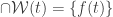
A collection of sets is said to be point-countable if every point in the space belongs to at most countably many sets in the collection. A base \mathcal{G} for a space X is said to be a point-countable base if \mathcal{G}, in addition to being a base for the space X, is also a point-countable collection of sets. The Michael line is an example of a space that has a point-countable base and that is not metrizable. The following is a point-countable base for \mathbb{M}:

    \mathcal{G}=\mathcal{H} \cup \left\{\left\{ x \right\}: x \in \mathbb{P}\right\}

where \mathcal{H} is the set of all Euclidean open intervals with rational endpoints. One reason for the interest in point-countable base is that any countable compact space (hence any compact space) with a point-countable base is metrizable (see Metrization Theorems for Compact Spaces).

___________________________________________________________________________________

Reference

  1. Engelking, R., General Topology, Revised and Completed edition, Heldermann Verlag, Berlin, 1989.
  2. Willard, S., General Topology, Addison-Wesley Publishing Company, 1970.

___________________________________________________________________________________

\copyright \ \ 2012

Alexandroff Double Circle

We discuss the Alexandroff double circle, which is a compact and non-metrizable space. A theorem about the hereditarily normality of a product space Y_1 \times Y_2 is also discussed.

Let C_1 and C_2 be the two concentric circles centered at the origin with radii 1 and 2, respectively. Specifically C_i=\left\{(x,y) \in \mathbb{R}^2: x^2 + y^2 =i \right\} where i=1,2. Let X=C_1 \cup C_2. Furthermore let f:C_1 \rightarrow C_2 be the natural homeomorphism. Figure 1 below shows the underlying set.

_______________________________________________________________
Figure 1 – Underlying Set

_______________________________________________________________

We define a topology on X as follows:

  • Points in C_2 are isolated.
  • For each x \in C_1 and for each positive integer j, let O(x,j) be the open arc in C_1 whose center contains x and has length \frac{1}{j} (in the Euclidean topology on C_1). For each x \in C_1, an open neighborhood is of the form B(x,j) where
      \text{ }

      B(x,j)=O(x,j) \cup (f(O(x,j))-\left\{f(x) \right\}).

    The following figure shows an open neighborhood at point in C_1.

_______________________________________________________________
Figure 2 – Open Neighborhood

___________________________________________________________________________________

A List of Results

It can be verified that the open neighborhoods defined above form a base for a topology on X. We discuss the following points about the Alexandroff double circle.

  1. X is a Hausdorff space.
  2. X is not separable.
  3. X is not hereditarily Lindelof.
  4. X is compact.
  5. X is sequentially compact.
  6. X is not metrizable.
  7. X is not perfectly normal.
  8. X is completely normal (and thus hereditarily normal).
  9. X \times X is not hereditarily normal.

The proof that X \times X is not hereditarily normal can be generalized. We discuss this theorem after presenting the proof of Result 9.
___________________________________________________________________________________

Results 1, 2, 3

It is clear that the Alexandroff double circle is a Hausdorff space. It is not separable since the outer circle C_2 consists of uncountably many singleton open subsets. For the same reason, C_2 is a non-Lindelof subspace, making the Alexandroff double circle not hereditarily Lindelof. \blacksquare

___________________________________________________________________________________

Result 4

The property that X is compact is closely tied to the compactness of the inner circle C_1 in the Euclidean topology. Note that the subspace topology of the Alexandroff double circle on C_1 is simply the Euclidean topology. Let \mathcal{U} be an open cover of X consisting of open sets as defined above. Then there are finitely many basic open sets B(x_1,j_1), B(x_2,j_2), \cdots, B(x_n,j_n) from \mathcal{U} covering C_1. These open sets cover the entire space except for the points f(x_1), f(x_2), \cdots,f(x_n), which can be covered by finitely many open sets in \mathcal{U}. \blacksquare

___________________________________________________________________________________

Result 5

A space W is sequentially compact if every sequence of points of W has a subsequence that converges to a point in W. The notion of sequentially compactness and compactness coincide for the class of metric spaces. However, in general these two notions are distinct.

The sequentially compactness of the Alexandroff double circle X hinges on the sequentially compactness of C_1 and C_2 in the Euclidean topology. Let \left\{x_n \right\} be a sequence of points in X. If the set \left\{x_n: n=1,2,3,\cdots \right\} is a finite set, then \left\{x_n: n>m \right\} is a constant sequence for some large enough integer m. So assume that A=\left\{x_n: n=1,2,3,\cdots \right\} is an infinite set. Either A \cap C_1 is infinite or A \cap C_2 is infinite. If A \cap C_1 is infinite, then some subsequence of \left\{x_n \right\} converges in C_1 in the Euclidean topology (hence in the Alexandroff double circle topology). If A \cap C_2 is infinite, then some subsequence of \left\{x_n \right\} converges to x \in C_2 in the Euclidean topology. Then this same subsequence converges to f^{-1}(x) in the Alexandroff double circle topology. \blacksquare

___________________________________________________________________________________

Result 6

Note that any compact metrizable space satisfies a long list of properties, which include separable, Lindelof, hereditarily Lindelof. \blacksquare

___________________________________________________________________________________

Result 7

A space is perfectly normal if it is normal with the additional property that every closed set is a G_\delta-set. For the Alexandroff double circle, the inner circle C_1 is not a G_\delta-set, or equivalently the outer circle C_2 is not an F_\sigma-set. To see this, suppose that C_2 is the union of countably many sets, we show that the closure of at least one of the sets goes across to the inner circle C_1. Let C_2=\bigcup \limits_{i=1}^\infty T_n. At least one of the sets is uncountable. Let T_j be one such. Consider f^{-1}(T_j), which is also uncountable and has a limit point in C_1 (in the Euclidean topology). Let t be one such point (i.e. every Euclidean open set containing t contains points of f^{-1}(T_j)). Then the point t is a member of the closure of T_j (Alexandroff double circle topology). \blacksquare

___________________________________________________________________________________

Result 8

We first discuss the notion of separated sets. Let T be a Hausdorff space. Let E \subset T and F \subset T. The sets E and F are said to be separated (are separated sets) if E \cap \overline{F}=\varnothing and F \cap \overline{E}=\varnothing. In other words, two sets are separated if each one does not meet the closure of the other set. In particular, any two disjoint closed sets are separated. The space T is said to be completely normal if T satisfies the property that for any two sets E and F that are separated, there are disjoint open sets U and V with E \subset U and F \subset V. Thus completely normality implies normality.

It is a well know fact that if a space is completely normal, it is hereditarily normal (actually the two notions are equivalent). Note that any metric space is completely normal. In particular, any Euclidean space is completely normal.

To show that the Alexandroff double circle X is completely normal, let E \subset X and F \subset X be separated sets. Thus we have E \cap \overline{F}=\varnothing and F \cap \overline{E}=\varnothing. Note that E \cap C_1 and F \cap C_1 are separated sets in the Euclidean space C_1. Let G_1 and G_2 be disjoint Euclidean open subsets of C_1 with E \cap C_1 \subset G_1 and F \cap C_1 \subset G_2.

For each x \in E \cap C_1, choose open U_x (Alexandroff double circle open) with x \in U_x, U_x \cap C_1 \subset G_1 and U_x \cap \overline{F}=\varnothing. Likewise, for each y \in F \cap C_1, choose open V_y (Alexandroff double circle open) with y \in V_y, V_y \cap C_1 \subset G_2 and V_y \cap \overline{E}=\varnothing. Then let U and V be defined by the following:

    U=\biggl(\bigcup \limits_{x \in E \cap C_1} U_x \biggr) \cup \biggl(E \cap C_2 \biggr)

    \text{ }

    V= \biggl(\bigcup \limits_{y \in F \cap C_1} V_y \biggr) \cup \biggl(F \cap C_2 \biggr)

Because G_1 \cap G_2 =\varnothing, the open sets U_x and V_y are disjoint. As a result, U and V are disjoint open sets in the Alexandroff double circle with E \subset U and F \subset V.

For the sake of completeness, we show that any completely normal space is hereditarily normal. Let T be completely normal. Let Y \subset T. Let H \subset Y and K \subset Y be disjoint closed subsets of Y. Then in the space T, H and K are separated. Note that H \cap cl_T(K)=\varnothing and K \cap cl_T(H)=\varnothing (where cl_T gives the closure in T). Then there are disjoint open subsets O_1 and O_2 of T such that H \subset O_1 and K \subset O_2. Now, O_1 \cap Y and O_2 \cap Y are disjoint open sets in Y such that H \subset O_1 \cap Y and K \subset O_2 \cap Y.

Thus we have established that the Alexandroff double circle is hereditarily normal. \blacksquare

For the proof that a space is completely normal if and only if it is hereditarily normal, see Theorem 2.1.7 in page 69 of [1],
___________________________________________________________________________________

Result 9

We produce a subspace Y \subset X \times X that is not normal. To this end, let D=\left\{d_n:n=1,2,3,\cdots \right\} be a countable subset of X such that \overline{D}-D\ne \varnothing. Let y \in \overline{D}-D. Let Y=X \times X-C_1 \times \left\{y \right\}. We show that Y is not normal.

Let H=C_1 \times (X-\left\{y \right\}) and K=C_2 \times \left\{y \right\}. These are two disjoint closed sets in Y. Let U and V be open in Y such that H \subset U and K \subset V. We show that U \cap V \ne \varnothing.

For each integer j, let U_j=\left\{x \in X: (x,d_j) \in U \right\}. We claim that each U_j is open in X. To see this, pick x \in U_j. We know (x,d_j) \in U. There exist open A and B (open in X) such that (x,d_j) \in A \times B \subset U. It is clear that x \in A \subset U_j. Thus each U_j is open.

Furthermore, we have C_1 \subset U_j for each j. Based in Result 7, C_1 is not a G_\delta-set. So we have C_1 \subset \bigcap \limits_{j=1}^\infty U_j but C_1 \ne \bigcap \limits_{j=1}^\infty U_j. There exists t \in \bigcap \limits_{j=1}^\infty U_j but t \notin C_1. Thus t \in C_2 and \left\{t \right\} is open.

Since (t,y) \in K, we have (t,y) \in V. Choose an open neighborhood B(y,k) of y such that \left\{t \right\} \times B(y,k) \subset V. since y \in \overline{D}, there exists some d_j such that (t,d_j) \in \left\{t \right\} \times B(y,k). Hence (t,d_j) \in V. Since t \in U_j, (t,d_j) \in U. Thus U \cap V \ne \varnothing. \blacksquare

___________________________________________________________________________________

Generalizing the Proof of Result 9

The proof of Result 9 requires that one of the factors has a countable set that is not discrete and the other factor has a closed set that is not a G_\delta-set. Once these two requirements are in place, we can walk through the same proof and show that the cross product is not hereditarily normal. Thus, the statement that is proved in Result 9 is the following.

Theorem
If Y_1 has a countable subset that is not closed and discrete and if Y_2 has a closed set that is not a G_\delta-set then Y_1 \times Y_2 has a subspace that is not normal.

The theorem can be restated as:

Theorem
If Y_1 \times Y_2 is hereditarily normal, then either every countable subset of Y_1 is closed and discrete or Y_2 is perfectly normal.

The above theorem is due to Katetov and can be found in [2]. It shows that the hereditarily normality of a cross product imposes quite strong restrictions on the factors. As a quick example, if both Y_1 and Y_2 are compact, for Y_1 \times Y_2 to be hereditarily normal, both Y_1 and Y_2 must be perfectly normal.

Another example. Let W=\omega_1+1, the succesor of the first uncountable ordinal with the order topology. Note that W is not perfectly normal since the point \omega_1 is not a G_\delta point. Then for any compact space Y, W \times Y is not hereditarily normal. Let C=\omega+1, the successor of the first infinite ordinal with the order topology (essentially a convergent sequence with the limit point). The product W \times C is the Tychonoff plank and based on the discussion here is not hereditarily normal. Usually the Tychonoff plank is shown to be not hereditarily normal by removing the cornor point (\omega_1,\omega). The resulting space is the deleted Tychonoff plank and is not normal (see The Tychonoff Plank).

___________________________________________________________________________________

Reference

  1. Engelking, R., General Topology, Revised and Completed edition, Heldermann Verlag, Berlin, 1989.
  2. Przymusinski, T. C., Handbook of Set-Theoretic Topology (K. Kunen and J. E. Vaughan, eds), Elsevier Science Publishers B. V., Amsterdam, 781-826, 1984.
  3. Willard, S., General Topology, Addison-Wesley Publishing Company, 1970.

___________________________________________________________________________________

\copyright \ \ 2012

Stone-Cech Compactifications – Another Two Characterizations

Let X be a completely regular space. Let \beta X be the Stone-Cech compactification of X. We present two characterizations of \beta X in addition to three others that are discussed previously. In all, these five characterizations can help us derive many of the basic properties of \beta X. We prove the following theorems.

Theorem C4
Let X be a completely regular space. Every two completely separated subsets of X have disjoint closures in \beta X.

Theorem U4
The property described in Theorem C4 is unique to \beta X. That is, if \alpha X is a compactification of X satisfying the condition that every two completely separated subsets of X have disjoint closures in \alpha X, then \alpha X must be \beta X.

Theorem C5
Let X be a normal space. Then every two disjoint closed subsets of X have disjoint closures in \beta X.

Theorem U5
If \alpha X is a compactification of X satisfying the property that every two disjoint closed subsets of X have disjoint closures in \alpha X, then X is normal and \alpha X must be \beta X.

The C theorem and U theorem with the same number work as a pair. The C theorem asserts that \beta X has a certain property. The corresponding U theorem asserts that of all the compactifications of X, \beta X is the only one with the property in question. Whenever we can show a given compactification does not possess the property described in the C-U theorem pair, we know that that compactification is not \beta X (consequence of the C theorem). Whenever we can show that a given compactification has the property described in the C-U theorem pair, we know that that compactification must be \beta X (a consequence of the U theorem).

Three other sets of characterizations (Theorems C1, U1, C2, U2, C3 and U3) have been established previously. See the links found below.
___________________________________________________________________________________

Completely Separated Sets

Let Y be a completely regular space. Let H \subset Y and K \subset Y. The sets H and K are said to be completely separated in Y if there is a continuous function f:Y \rightarrow [0,1] such that for each y \in H, f(y)=0 and for each y \in K, f(y)=1 (this can also be expressed as f(H) \subset \left\{0 \right\} and f(K) \subset \left\{1 \right\}). If H and K are completely separated, \overline{H} and \overline{K} are necessarily disjoint closed sets, since \overline{H} \subset f^{-1}(0) and \overline{K} \subset f^{-1}(1).

The Urysohn’s lemma can be stated as: a space is a normal space if and only if every two disjoint closed sets are completely separated. Thus disjoint closed sets are not necessarily completely separated (such sets can be found in non-normal spaces).

___________________________________________________________________________________

Some Helpful Results

To prove Theorem U4, we need a lemma and a theorem. Most of the work in proving Theorem U4 is carried out in Theorem 2 below.

Lemma 1
Let Y be a compact space. Let U be an open subset of Y. Let \mathcal{C} be a collection of compact subsets of Y such that \cap \mathcal{C} \subset U. Then there exists a finite collection \left\{C_1,C_2,\cdots,C_n \right\} \subset \mathcal{C} such that \bigcap \limits_{i=1}^n C_i \subset U.

Proof of Lemma 1
Let D=Y-U, which is compact. Let \mathcal{O} be the collection of all Y-C where C \in \mathcal{C}. Note that \cap \mathcal{C} \subset U implies that D \subset \cup \mathcal{O}. Thus \mathcal{O} is a collection of open sets covering the compact set D. We have \left\{O_1,O_2,\cdots,O_n \right\} \subset \mathcal{O} such that D \subset \bigcup \limits_{i=1}^n O_i. Each O_i=Y-C_i for some C_i \in \mathcal{C}. Now \left\{C_1,C_2,\cdots,C_n \right\} is the desired finite collection. \blacksquare

Theorem 2
Let T be a completely regular space. Let S be a dense subspace of T. Let f:S \rightarrow K be a continuous function from S into a compact space K. Suppose that every two completely separated subsets of S have disjoint closures in T. Then f can be extended to a continuous F:T \rightarrow K.

Proof
For each t \in T, let \mathcal{O}(t) be the set of all open subsets of T containing t. For each t \in T, let \mathcal{W}(t) be the set of all \overline{f(S \cap O)} where O \in \mathcal{O}(t). Note that each \mathcal{W}(t) consists of compact subsets of K. The theorem is established by proving the following claims.

Claim 1
For each t \in T, the collection \mathcal{W}(t) has non-empty intersection.

For any O_1, O_2, \cdots, O_n \in \mathcal{O}(t), we have the following:

    \overline{f(S \cap O_1 \cap O_2 \cap \cdots \cap O_n)} \subset \overline{f(S \cap O_1)} \cap \overline{f(S \cap O_2)} \cap \cdots \cap \overline{f(S \cap O_n)}

The above shows that \mathcal{W}(t) has the finite intersection property (f. i. p.). It is a well known fact that in a compact space, any collection of sets with f. i. p. has non-empty intersection (see [1] or [2] or see The Finite Intersection Property in Compact Spaces and Countably Compact Spaces in this blog).

Claim 2
For each t \in T, \cap \mathcal{W}(t) has only one point.

Let t \in T. Suppose that

    \left\{k_1,k_2 \right\} \subset \cap \mathcal{W}(t) where k_1 \ne k_2 \ \ \ \ \ \ \ \ \ \ \ \ \ \ (1)

Then there exist open subsets U_1 and U_2 of K such that k_1 \in U_1, k_2 \in U_2 and \overline{U_1} \cap \overline{U_2} = \varnothing. Since K is compact, it is a normal space. By the Urysohn’s lemma, there exists a continuous g:K \rightarrow [0,1] such that for each k \in \overline{U_1}, g(k)=0 and for each k \in \overline{U_2}, g(k)=1. Then because of the function g \circ f:S \rightarrow [0,1], the sets f^{-1}(\overline{U_1}) and f^{-1}(\overline{U_2}) are completely separated sets in S. By assumption, these two sets have disjoint closures in T, i.e.,

    \text{ }
    \overline{f^{-1}(\overline{U_1})} \cap \overline{f^{-1}(\overline{U_2})} = \varnothing \ \ \ \ \ \ \ \ \ \ \ \ \ \ \ \ \ \ \ \ \ \ \ (2)
    \text{ }

The point t cannot be in both of the sets in (2). Assume the following:

    \text{ }
    t \notin \overline{f^{-1}(\overline{U_1})} \ \ \ \ \ \ \ \ \ \ \ \ \ \ \ \ \ \ \ \ \ \ \ \ \ \ \ \ \ \ \ \ \ \ \ \ \ \ (3)
    \text{ }

Then H=T- \overline{f^{-1}(\overline{U_1})} \in \mathcal{O}(t). Note that S \cap H=S-\overline{f^{-1}(\overline{U_1})}. Furthermore, \overline{f(S-\overline{f^{-1}(\overline{U_1})})} \in \mathcal{W}(t). Thus we have:

    \text{ }
    k_1 \in \cap \mathcal{W}(t) \subset \overline{f(S-\overline{f^{-1}(\overline{U_1})})}=W
    \text{ }

Since k_1 \in W and U_1 is an open set containing k_1, U_1 contains at least one point of f(S-\overline{f^{-1}(\overline{U_1})}). Choose z \in U_1 such that z \in f(S-\overline{f^{-1}(\overline{U_1})}). Now choose a \in S-\overline{f^{-1}(\overline{U_1})} such that f(a)=z. First we have a \notin \overline{f^{-1}(\overline{U_1})} and thus a \notin f^{-1}(\overline{U_1}). Secondly since f(a)=z \in U_1, we have a \in f^{-1}(U_1) \subset f^{-1}(\overline{U_1}). We now have a \notin f^{-1}(\overline{U_1}) and a \in f^{-1}(\overline{U_1}), a contradiction. If we assume t \notin \overline{f^{-1}(\overline{U_2})}, we can also derive a contradiction in a similar derivation. Thus the assumption in (1) above is faulty. The intersection \cap \mathcal{W}(t) can only have one point.

Claim 3
For each t \in S, \cap \mathcal{W}(t) =\left\{f(t) \right\}.

Let t \in S. Suppose that \cap \mathcal{W}(t) =\left\{p \right\} where p \ne f(t). the rest of the proof for Claim 3 is similar to that of Claim 2. For the sake of completeness, we give a sketch.

There exist open subsets U_1 and U_2 of K such that p \in U_1, f(t) \in U_2 and \overline{U_1} \cap \overline{U_2} = \varnothing. By the same argument as in Claim 2, we have the condition (2), i.e., \overline{f^{-1}(\overline{U_1})} \cap \overline{f^{-1}(\overline{U_2})} = \varnothing. Since t \in f^{-1}(U_2), t \notin \overline{f^{-1}(\overline{U_1})}. The remainder of the proof of Claim 3 is the same as above starting with condition (3) with p=k_1. A contradiction will be obtained. We can conclude that the assumption that \cap \mathcal{W}(t) =\left\{p \right\} where p \ne f(t) must be faulty. Thus Claim 3 is established.

Claim 4
For each t \in T, define F:T \rightarrow K by letting F(t) be the point in \cap \mathcal{W}(t). Note that this function extends f. Furthermore, the map F:T \rightarrow K is continuous.

To show F is continuous, let t \in T and let F(t) \in E where E is open in K. The collection \mathcal{W}(t) is a collection of compact subsets of K such that \left\{F(t) \right\} =\cap \mathcal{W}(t) \subset E. By Lemma 1, there exists \left\{C_1,\cdots,C_n \right\} \subset \mathcal{W}(t) such that \bigcap \limits_{i=1}^n C_i \subset E. By the definition of \mathcal{W}(t), there exists \left\{O_1,O_2,\cdots,O_n \right\} \subset \mathcal{O}(t) such that each C_i=\overline{f(S \cap O_i)}. Let O=O_1 \cap O_2 \cap \cdots \cap O_n. We have:

    \text{ }
    \overline{f(S \cap O)} \subset \bigcap \limits_{i=1}^n \overline{f(S \cap O_i)} \subset E \ \ \ \ \ \ \ \ \ \ \ \ \ \ (4)
    \text{ }

Note that O 
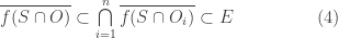
is an open subset of T and t \in O. We show that F(O) \subset E. Pick a \in O. According to the definition of \mathcal{W}(a), we have \left\{F(a) \right\}=\bigcap \limits_{U \in \mathcal{O}(a)} \overline{f(S \cap U)}. Since O \in \mathcal{O}(a), we have F(a) \in \overline{f(S \cap O)}. Thus by (4), we have F(a) \in E. Thus Claim 4 is established.

With all the above claims established, we completed the proof of Theorem 2. \blacksquare

___________________________________________________________________________________

Theorem C4 and Theorem U4

Proof of Theorem C4
In proving C4, we use Theorem C3, which is found in C*-Embedding Property and Stone-Cech Compactification.

Let E and F be two completely separated sets in X. Then there exists some continuous g:X \rightarrow [0,1] such that for each x \in E, g(x)=0 and for each x \in F, g(x)=1. By Theorem C3, g is extended by some continuous G:\beta X \rightarrow [0,1]. The sets G^{-1}(0) and G^{-1}(1) are disjoint closed sets in \beta X. Furthermore, E \subset G^{-1}(0) and F \subset G^{-1}(1). Thus E and F have disjoint closures in \beta X. \blacksquare

Proof of Theorem U4
In proving U4, we use Theorem U1, which is stated and proved in Two Characterizations of Stone-Cech Compactification.

Suppose that \alpha X is a compactification of X satisfying the condition that every two completely separated subsets of X have disjoint closures in \alpha X. Let g:X \rightarrow Y be a continuous function from X into a compact space Y. By Theorem 2, g can be extended by a continuous G:\alpha X \rightarrow Y. By Theorem U1, \alpha X must be \beta X. \blacksquare

___________________________________________________________________________________

Theorem C5 and Theorem U5

Proof of Theorem C5
Let X be a normal space. According to the Urysohn’s lemma, every two disjoint closed sets are completely separated. Thus by Theorem C4, every two disjoint closed subsets of X have disjoint closures in \beta X. \blacksquare

Proof of Theorem U5
Suppose that \alpha X is a compactification of X satisfying the property that every two disjoint closed subsets of X have disjoint closures in \alpha X. To show that X is normal, let H and K be disjoint closed subsets of X. By assumption about \alpha X, \overline{H} and \overline{K} (closures in \alpha X) are disjoint. Since \alpha X are compact and Hausdorff, \alpha X is normal. Then \overline{H} and \overline{K} can be separated by disjoint open subsets U and V of \alpha X. Thus U \cap X and V \cap X are disjoint open subsets of X separating H and K.

We use Theorem U4 to prove Theorem U5. We show that \alpha X satisfies Theorem U4. To this end, let E and F be two completely separated sets in X. We show that E and F have disjoint closures in \alpha X. There exists some continuous f:X \rightarrow [0,1] such that for each x \in E, f(x)=0 and for each x \in F, f(x)=1. Then f^{-1}(0) and f^{-1}(1) are disjoint closed sets in X such that E \subset f^{-1}(0) and F \subset f^{-1}(1). By assumption about \alpha X, f^{-1}(0) and f^{-1}(1) have disjoint closures in \alpha X. This implies that E and F have disjoint closures in \alpha X. Then by Theorem U4, \alpha X must be \beta X. \blacksquare

___________________________________________________________________________________

Blog Posts on Stone-Cech Compactification

___________________________________________________________________________________

Reference

  1. Engelking, R., General Topology, Revised and Completed edition, Heldermann Verlag, Berlin, 1989.
  2. Willard, S., General Topology, Addison-Wesley Publishing Company, 1970.

___________________________________________________________________________________

\copyright \ \ 2012

Stone-Cech Compactification of the Integers – Basic Facts

This is another post Stone-Cech compactification. The links for other posts on Stone-Cech compactification can be found below. In this post, we prove a few basic facts about \beta \omega, the Stone-Cech compactification of the discrete space of the non-negative integers, \omega=\left\{0,1,2,3,\cdots \right\}. We use several characterizations of Stone-Cech compactification to find out what \beta \omega is like. These characterizations are proved in the blog posts listed below. Let c denote the cardinality of the real line \mathbb{R}. We prove the following facts.

  1. The cardinality of \beta \omega is 2^c.
  2. The weight of \beta \omega is c.
  3. The space \beta \omega is zero-dimensional.
  4. Every infinite closed subset of \beta \omega contains a topological copy of \beta \omega.
  5. The space \beta \omega contains no non-trivial convergent sequence.
  6. No point of \beta \omega-\omega is an isolated point.
  7. The space \beta \omega fails to have many properties involving the existence of non-trivial convergent sequence. For example:
    \text{ }

    1. The space \beta \omega is not first countable at each point of the remainder \beta \omega-\omega.
    2. The space \beta \omega is not a Frechet space.
    3. The space \beta \omega is not a sequential space.
    4. The space \beta \omega is not sequentially compact.

    \text{ }

  8. No point of the remainder \beta \omega-\omega is a G_\delta-point.
  9. The remainder \beta \omega-\omega does not have the countable chain condition. In fact, it has a disjoint open collection of cardinality c.

___________________________________________________________________________________

Characterization Theorems

For any completely regular space X, let C(X,I) be the set of all continuous functions from X into I=[0,1]. The Stone-Cech compactification \beta X is the subspace of the product space [0,1]^{C(X,I)} which is the closure of the image of X under the evaluation map \beta:X \rightarrow [0,1]^{C(X,I)} (for the details, see Embedding Completely Regular Spaces into a Cube).

The brief sketch of \beta \omega we present here is not based on the definition using the evaluation map. Instead we reply on some characterization theorems that are stated here (especially Theorem U3.1). These theorems uniquely describe the Stone-Cech compactification \beta X of a given completely regular space X. For example, \beta X satisfies the function extension property in Theorem C3 below. Furthermore any compactification \alpha X of X that satisfies the same property must be \beta X (Theorem U3.1). So a “C” theorem tells us a property possessed by \beta X. The corresponding “U” theorem tells us that there is only one compactification (up to equivalence) that has this property.

    _______________________________________________________________________________________
    Theorem C1
    Let X be a completely regular space. Let f:X \rightarrow Y be a continuous function from X into a compact Hausdorff space Y. Then there is a continuous F: \beta X \rightarrow Y such that F \circ \beta=f.

    \text{ }

    Theorem C2
    Let X be a completely regular space. Among all compactifications of the space X, the Stone-Cech compactification \beta X of the space X is maximal with respect to the partial order \le.

    \text{ }

    Theorem U2
    The property in Theorem C2 is unique to \beta X. That is, if, among all compactifications of the space X, \alpha X is maximal with respect to the partial order \le, then \alpha X \approx \beta X.

    See Two Characterizations of Stone-Cech Compactification.
    _______________________________________________________________________________________
    \text{ }

    Theorem C3
    Let X be a completely regular space. The space X is C^*-embedded in its Stone-Cech compactification \beta X.

    \text{ }

    Theorem U3.1
    Let X be a completely regular space. Let I=[0,1]. Let \alpha X be a compactification of X such that each continuous f:X \rightarrow I can be extended to a continuous \hat{f}:\alpha X \rightarrow I. Then \alpha X must be \beta X.

    \text{ }

    Theorem U3.2
    If \alpha X is any compactification of X that satisfies the property in Theorem C3 (i.e., X is C^*-embedded in \alpha X), then \alpha X must be \beta X.

    See C*-Embedding Property and Stone-Cech Compactification.
    _______________________________________________________________________________________
    \text{ }

The following discussion illustrates how we can use some of these characterizations theorem to obtain information about \beta X and \beta \omega in particular.

___________________________________________________________________________________

Result 1 and Result 2

According to the previous post (Stone-Cech Compactification is Maximal), we have for any completely regular space X, \lvert \beta X \lvert \le 2^{2^{d(X)}} where d(X) is the density (the smallest cardinality of a dense set in X). With \omega being a countable space, \lvert \beta \omega \lvert \le 2^{2^{\omega}}=2^c.

Result 1 is established if we have 2^c \le \lvert \beta \omega \lvert. Consider the cube I^I where I is the unit interval I=[0,1]. Since the product space of c many separable space is separable (see Product of Separable Spaces), I^I is separable. Let S \subset I^I be a countable dense set. Let f:\omega \rightarrow S be a bijection. Clearly f is a continuous function from the discrete space \omega into I^I. By Theorem C1, f is extended by a continuous F:\beta \omega \rightarrow I^I. Note that the image F(\beta \omega) is dense in I^I since F(\beta \omega) contains the dense set S. On the other hand, F(\beta \omega) is compact. So F(\beta \omega)=I^I. Thus F is a surjection. The cardinality of I^I is 2^c. Thus we have 2^c \le \lvert \beta \omega \lvert.

From the same previous post (Stone-Cech Compactification is Maximal), it is shown that w(\beta X) \le 2^{d(X)}. Thus w(\beta \omega) \le 2^{\omega}=c. The same function F:\beta \omega \rightarrow I^I in the above paragraph shows that c \le w(\beta \omega) (see Lemma 2 in Stone-Cech Compactification is Maximal). Thus we have w(\beta \omega)=c \blacksquare

___________________________________________________________________________________

Result 3

A space is said to be zero-dimensional whenever it has a base consisting of open and closed sets. The proof that \beta X is zero-dimensional comes after the following lemmas and theorems.

    Theorem 1
    Let X be a normal space. If H and K are disjoint closed subsets of X, then H and K have disjoint closures in \beta X.

Proof of Theorem 1
Let H and K be disjoint closed subsets of X. By the normality of X and by the Urysohn’s lemma, there is a continuous function g:X \rightarrow [0,1] such that g(H) \subset \left\{0 \right\} and g(K) \subset \left\{1 \right\}. By Theorem C3.1, g can be extended by G:\beta X \rightarrow [0,1]. Note that \overline{H} \subset G^{-1}(0) and \overline{K} \subset G^{-1}(1). Thus \overline{H} \cap \overline{K} = \varnothing. \blacksquare

    Theorem 2
    Let X be a completely regular space. Let H be a closed and open subset of X. Then \overline{H} (the closure of H in \beta X) is also a closed and open set in \beta X.

Proof of Theorem 2
Let H be a closed and open subset of X. Let K=X-H. Define \gamma:X \rightarrow [0,1] by letting \gamma(x)=0 for all x \in H and \gamma(x)=1 for all x \in K. Since both H and K are closed and open, the map \gamma is continuous. By Theorem C3, \gamma is extended by some continuous \Gamma:\beta X \rightarrow [0,1]. Note that \overline{H} \subset \Gamma^{-1}(0) and \overline{K} \subset \Gamma^{-1}(1). Thus H and K have disjoint closures in \beta X, i.e. \overline{H} \cap \overline{K} = \varnothing. Both H and K are closed and open in \beta X since \beta X=\overline{H} \cup \overline{K}. \blacksquare

    Lemma 3
    For every A \subset \omega, \overline{A} (the closure of A in \beta \omega) is both closed and open in \beta \omega.

Note that Lemma 3 is a corollary of Theorem 2.

    Lemma 4
    Let O \subset \beta \omega be a set that is both closed and open in \beta \omega. Then O=\overline{A} where A= O \cap \omega.

Proof of Lemma 4
Let A=O \cap \omega. Either O \subset \omega or O \cap (\beta \omega-\omega) \ne \varnothing. Thus A \ne \varnothing. We claim that O=\overline{A}. Since A \subset O, it follows that \overline{A} \subset \overline{O}=O. To show O \subset \overline{A}, pick x \in O. If x \in \omega, then x \in A. So focus on the case that x \notin \omega. It is clear that x \notin \overline{B} where B=\omega -A. But every open set containing x must contain some points of \omega. These points of \omega must be points of A. Thus we have x \in \overline{A}. \blacksquare

Proof of Result 3
Let \mathcal{A} be the set of all closed and open sets in \beta \omega. Let \mathcal{B}=\left\{\overline{A}: A \subset \omega \right\}. Lemma 3 shows that \mathcal{B} \subset \mathcal{A}. Lemma 4 shows that \mathcal{A} \subset \mathcal{B}. Thus \mathcal{A}= \mathcal{B}. We claim that \mathcal{B} is a base for \beta \omega. To this end, we show that for each open O \subset \beta \omega and for each x \in O, we can find \overline{A} \in \mathcal{B} with x \in \overline{A} \subset O. Let O be open and let x \in O. Since \beta \omega is a regular space, we can find open set V \subset \beta \omega with x \in V \subset \overline{V} \subset O. Let A=V \cap \omega.

We claim that x \in \overline{A}. Suppose x \notin \overline{A}. There exists open U \subset V such that x \in U and U misses \overline{A}. But U must meets some points of \omega, say, y \in U \cap \omega. Then y \in V \cap \omega=A, which is a contradiction. So we have x \in \overline{A}.

It is now clear that x \in \overline{A} \subset \overline{V} \subset O. Thus \beta \omega is zero-dimensional since \mathcal{B} is a base consisting of closed and open sets. \blacksquare

___________________________________________________________________________________

Result 4 and Result 5

Result 5 is a corollary of Result 4. We first prove two lemmas before proving Result 4.

    Lemma 5
    For each infinite A \subset \omega, \overline{A} (the closure of A in \beta \omega) is a homeomorphic copy of \beta \omega and thus has cardinality 2^c.

Proof of Lemma 5
Let A \subset \omega. Let g:A \rightarrow [0,1] be any function (necessarily continuous). Let f:\omega \rightarrow [0,1] be defined by f(x)=g(x) for all x \in A and f(x)=0 for all x \in \omega-A. By Theorem C3, f can be extended by F:\beta \omega \rightarrow [0,1]. Let G=F \upharpoonright \overline{A}.

Note that the function G: \overline{A} \rightarrow [0,1] extends g:A \rightarrow [0,1]. Thus by Theorem U3.1, \overline{A} must be \beta A. Since A is a countably infinite discrete space, \beta A must be equivalent to \beta \omega. \blacksquare

    Lemma 6
    For each countably infinite A \subset \beta \omega-\omega such that A is relatively discrete, \overline{A} (the closure of A in \beta \omega) is a homeomorphic copy of \beta \omega and thus has cardinality 2^c.

Proof of Lemma 6
Let A=\left\{t_1,t_2,t_3,\cdots \right\} \subset \beta \omega -\omega such that A is discrete in the relative topology inherited from \beta \omega. There exist disjoint open sets G_1,G_2,G_3,\cdots (open in \beta \omega) such that for each j, t_j \in G_j. Since \beta \omega is zero-dimensional (Result 3), G_1,G_2,G_3,\cdots can be made closed and open.

Let f:A \rightarrow [0,1] be a continuous function. We show that f can be extended by F:\overline{A} \rightarrow [0,1]. Once this is shown, by Theorem U3.1, \overline{A} must be \beta A. Since A is a countable discrete space, \beta A must be equivalent to \beta \omega.

We first define w:\omega \rightarrow [0,1] by:

    \displaystyle w(n)=\left\{\begin{matrix}f(t_j)& \exists \ j \text{ such that } n \in \omega \cap G_j\\{0}&\text{otherwise} \end{matrix}\right.

The function w 
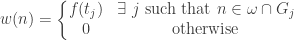
is well defined since each n \in \omega is in at most one G_j. By Theorem C3, the function w is extended by some continuous W:\beta \omega \rightarrow [0,1]. By Lemma 4, for each j, G_j=\overline{\omega \cap G_j}. Thus, for each j, t_j \in \overline{\omega \cap G_j}. Note that W is a constant function on the set \omega \cap G_j (mapping to the constant value of f(t_j)). Thus W(t_j)=f(t_j) for each j. So let F=W \upharpoonright \overline{A}. Thus F is the desired function that extends f. \blacksquare

Proof of Result 4
Let C \subset \beta \omega be an infinite closed set. Either C \cap \omega is infinite or C \cap (\beta \omega-\omega) is infinite. If C \cap \omega is infinite, then by Lemma 5, \overline{C \cap \omega} is a homeomorphic copy of \beta \omega. Now focus on the case that C_0=C \cap (\beta \omega-\omega) is infinite. We can choose inductively a countably infinite set A \subset C_0 such that A is relatively discrete. Then by Lemma 6 \overline{A} is a copy of \beta \omega that is a subset of C. \blacksquare

___________________________________________________________________________________

Result 6

We prove that no point in the remainder \beta \omega-\omega is an isolated point. To see this, pick x \in \beta \omega-\omega and pick an arbitrary closed and open set O \subset \beta \omega with x \in O. Let V=O \cap (\beta \omega-\omega) (thus an arbitrary open set in the remainder containing x). By Lemma 4, O=\overline{A} where A=O \cap \omega. According to Lemma 5, O=\overline{A} is a copy of \beta \omega and thus has cardinality 2^c. The set V is O minus a subset of \omega. Thus V must contains 2^c many points. This means that \left\{ x \right\} can never be open in the remainder \beta \omega-\omega. In fact, we just prove that any open and closed subset of \beta \omega-\omega (thus any open subset) must have cardinality at least 2^c. \blacksquare

___________________________________________________________________________________

Result 7

The results under Result 7 are corollary of Result 5 (there is no non-trivial convergent sequence in \beta \omega). To see Result 7.1, note that every point x in the remainder is not an isolated point and hence cannot have a countable local base (otherwise there would be a non-trivial convergent sequence converging to x).

A space Y is said to be a Frechet space if A \subset Y and for each x \in \overline{A}, there is a sequence \left\{ x_n \right\} of points of A such that x_n \rightarrow x. A set A \subset Y is said to be sequentially closed in Y if for any sequence \left\{ x_n \right\} of points of A, x_n \rightarrow x implies x \in A. A space Y is said to be a sequential space if A \subset Y is a closed set if and only if A is a sequentially closed set. If a space is Frechet, then it is sequential. It is clear that \beta \omega is not a sequential space.

A space is said to be sequentially compact if every sequence of points in this space has a convergent subsequence. Even though \beta \omega is compact, it cannot be sequentially compact.

___________________________________________________________________________________

Result 8

Result 7.1 indicates that no point of remainder \beta \omega-\omega can have a countable local base. In fact, no point of the remainder can be a G_\delta-point (a point that is the intersection of countably many open sets). The remainder \beta \omega-\omega is a compact space (being a closed subset of \beta \omega). In a compact space, if a point is a G_\delta-point, then there is a countable local base at that point (see 3.1.F (a) on page 135 of [1] or 17F.7 on page 125 of [2]). \blacksquare

___________________________________________________________________________________

Result 9

The space \beta \omega is a separable space since \omega is a dense set. Thus \beta \omega has the countable chain condition. However, the remainder \beta \omega-\omega does not have the countable chain condition. We show that there is a disjoint collection of c many open sets in \beta \omega-\omega.

There is a family \mathcal{A} of infinite subsets of \omega such that for every A,B \in \mathcal{A} with A \ne B, A \cap B is finite. Such a collection of sets is said to be an almost disjoint family. There is even an almost disjoint family of cardinality c (see A Space with G-delta Diagonal that is not Submetrizable). Let \mathcal{A} be such a almost disjoint family.

For each A \in \mathcal{A}, let U_A=\overline{A} and V_A=\overline{A} \cap (\beta \omega -\omega). By Lemma 3, each U_A is a closed and open set in \beta \omega. Thus each V_A is a closed and open set in the remainder \beta \omega-\omega. Note that \left\{V_A: A \in \mathcal{A} \right\} is a disjoint collection of open sets in \beta \omega-\omega. \blacksquare

___________________________________________________________________________________

Blog Posts on Stone-Cech Compactification

___________________________________________________________________________________

Reference

  1. Engelking, R., General Topology, Revised and Completed edition, Heldermann Verlag, Berlin, 1989.
  2. Willard, S., General Topology, Addison-Wesley Publishing Company, 1970.

___________________________________________________________________________________

\copyright \ \ 2012