We discuss the Alexandroff double circle, which is a compact and non-metrizable space. A theorem about the hereditarily normality of a product space  is also discussed.
Let  and
and  be the two concentric circles centered at the origin with radii 1 and 2, respectively. Specifically
  where
where  . Let
. Let  . Furthermore let
  be the natural homeomorphism. Figure 1 below shows the underlying set.
_______________________________________________________________
Figure 1 – Underlying Set

_______________________________________________________________
We define a topology on  as follows:
The following figure shows an open neighborhood at point in .
_______________________________________________________________
Figure 2 – Open Neighborhood

___________________________________________________________________________________
A List of Results
It can be verified that the open neighborhoods defined above form a base for a topology on . We discuss the following points about the Alexandroff double circle.
- is a Hausdorff space.
- is not separable.
- is not hereditarily Lindelof.
- is compact.
- is sequentially compact.
- is not metrizable.
- is not perfectly normal.
- is completely normal (and thus hereditarily normal).
 is not hereditarily normal.
The proof that is not hereditarily normal can be generalized. We discuss this theorem after presenting the proof of Result 9.
___________________________________________________________________________________
Results 1, 2, 3
It is clear that the Alexandroff double circle is a Hausdorff space. It is not separable since the outer circle consists of uncountably many singleton open subsets. For the same reason, is a non-Lindelof subspace, making the Alexandroff double circle not hereditarily Lindelof. 
___________________________________________________________________________________
Result 4
The property that is compact is closely tied to the compactness of the inner circle in the Euclidean topology. Note that the subspace topology of the Alexandroff double circle on is simply the Euclidean topology. Let  be an open cover of consisting of open sets as defined above. Then there are finitely many basic open sets
  ,
,  ,
,  ,
,  from covering . These open sets cover the entire space except for the points
  , which can be covered by finitely many open sets in .
___________________________________________________________________________________
Result 5
A space  is sequentially compact if every sequence of points of has a subsequence that converges to a point in . The notion of sequentially compactness and compactness coincide for the class of metric spaces. However, in general these two notions are distinct.
The sequentially compactness of the Alexandroff double circle hinges on the sequentially compactness of and in the Euclidean topology. Let  be a sequence of points in . If the set
  is a finite set, then
  is a constant sequence for some large enough integer
  . So assume that
  is an infinite set. Either
  is infinite or
  is infinite. If is infinite, then some subsequence of converges in in the Euclidean topology (hence in the Alexandroff double circle topology). If is infinite, then some subsequence of converges to
  in the Euclidean topology. Then this same subsequence converges to
  in the Alexandroff double circle topology.
___________________________________________________________________________________
Result 6
Note that any compact metrizable space satisfies a long list of properties, which include separable, Lindelof, hereditarily Lindelof.
___________________________________________________________________________________
Result 7
A space is perfectly normal if it is normal with the additional property that every closed set is a  -set. For the Alexandroff double circle, the inner circle is not a -set, or equivalently the outer circle is not an
  -set. To see this, suppose that is the union of countably many sets, we show that the closure of at least one of the sets goes across to the inner circle . Let
  . At least one of the sets is uncountable. Let
  be one such. Consider
  , which is also uncountable and has a limit point in (in the Euclidean topology). Let
  be one such point (i.e. every Euclidean open set containing contains points of ). Then the point is a member of the closure of (Alexandroff double circle topology).
___________________________________________________________________________________
Result 8
We first discuss the notion of separated sets. Let  be a Hausdorff space. Let
  and
and  . The sets
  and
and  are said to be separated (are separated sets) if
  and
and  . In other words, two sets are separated if each one does not meet the closure of the other set. In particular, any two disjoint closed sets are separated. The space is said to be completely normal if satisfies the property that for any two sets and that are separated, there are disjoint open sets
  and
and  with
with  and
and  . Thus completely normality implies normality.
It is a well know fact that if a space is completely normal, it is hereditarily normal (actually the two notions are equivalent). Note that any metric space is completely normal. In particular, any Euclidean space is completely normal.
To show that the Alexandroff double circle is completely normal, let  and
and  be separated sets. Thus we have and . Note that
  and
and  are separated sets in the Euclidean space . Let
  and
and  be disjoint Euclidean open subsets of with
  and
and  .
.
For each  , choose open
  (Alexandroff double circle open) with
  ,
,  and
and  . Likewise, for each
  , choose open
  (Alexandroff double circle open) with
  ,
,  and
and  . Then let and be defined by the following:
Because  , the open sets and are disjoint. As a result, and are disjoint open sets in the Alexandroff double circle with and .
For the sake of completeness, we show that any completely normal space is hereditarily normal. Let be completely normal. Let  . Let
. Let  and
and  be disjoint closed subsets of
  . Then in the space ,
  and
and  are separated. Note that
  and
and  (where
  gives the closure in ). Then there are disjoint open subsets
  and
and  of such that
  and
and  . Now,
  and
and  are disjoint open sets in such that
  and
and  .
.
Thus we have established that the Alexandroff double circle is hereditarily normal.
For the proof that a space is completely normal if and only if it is hereditarily normal, see Theorem 2.1.7 in page 69 of [1],
___________________________________________________________________________________
Result 9
We produce a subspace  that is not normal. To this end, let
  be a countable subset of such that
  . Let
. Let  . Let
. Let  . We show that is not normal.
Let  and
and  . These are two disjoint closed sets in . Let and be open in such that
  and
and  . We show that
  .
.
For each integer  , let
, let  . We claim that each
  is open in . To see this, pick
  . We know
  . There exist open
  and
and  (open in ) such that
  . It is clear that
  . Thus each is open.
Furthermore, we have  for each . Based in Result 7, is not a -set. So we have
  but
but  . There exists
  but
but  . Thus
  and
and  is open.
Since  , we have
  . Choose an open neighborhood
  of
of  such that
  . since
  , there exists some
  such that
  . Hence
  . Since
  ,
,  . Thus .
___________________________________________________________________________________
Generalizing the Proof of Result 9
The proof of Result 9 requires that one of the factors has a countable set that is not discrete and the other factor has a closed set that is not a -set. Once these two requirements are in place, we can walk through the same proof and show that the cross product is not hereditarily normal. Thus, the statement that is proved in Result 9 is the following.
Theorem
If  has a countable subset that is not closed and discrete and if
  has a closed set that is not a -set then has a subspace that is not normal.
The theorem can be restated as:
Theorem
If is hereditarily normal, then either every countable subset of is closed and discrete or is perfectly normal.
The above theorem is due to Katetov and can be found in [2]. It shows that the hereditarily normality of a cross product imposes quite strong restrictions on the factors. As a quick example, if both and are compact, for to be hereditarily normal, both and must be perfectly normal.
Another example. Let  , the succesor of the first uncountable ordinal with the order topology. Note that is not perfectly normal since the point
  is not a point. Then for any compact space ,
  is not hereditarily normal. Let
  , the successor of the first infinite ordinal with the order topology (essentially a convergent sequence with the limit point). The product
  is the Tychonoff plank and based on the discussion here is not hereditarily normal. Usually the Tychonoff plank is shown to be not hereditarily normal by removing the cornor point
  . The resulting space is the deleted Tychonoff plank and is not normal (see The Tychonoff Plank).
___________________________________________________________________________________
Reference
- Engelking, R., General Topology, Revised and Completed edition, Heldermann Verlag, Berlin, 1989.
- Przymusinski, T. C., Handbook of Set-Theoretic Topology (K. Kunen and J. E. Vaughan, eds), Elsevier Science Publishers B. V., Amsterdam, 781-826, 1984.
- Willard, S., General Topology, Addison-Wesley Publishing Company, 1970.
___________________________________________________________________________________

![I=[0,1]](https://s0.wp.com/latex.php?latex=I%3D%5B0%2C1%5D&bg=ffffff&fg=333333&s=0&c=20201002)


is normal.


![E_n=(p_n,q_n]=(p_n,1]](https://s0.wp.com/latex.php?latex=E_n%3D%28p_n%2Cq_n%5D%3D%28p_n%2C1%5D&bg=ffffff&fg=333333&s=0&c=20201002)


 is the product of
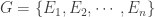
  where
where  cannot be hereditarily normal as long as there are uncountably many factors and every factor has at least two point.
 and
and  are hereditarily normal can tell us whether
  is not metrizable since it is not first countable (see Problem 1 below). Thus one of its first three self products must fail to be hereditarily normal.
  , let
, let  be a set with cardinality
  . Show that
  .
. be a space with at least two points. Show that for every point
  , there does not exist a countable base at the point
  . In other words, the product space
  is not first countable at every point. It follows that product space
  is a
is a  and that it has only finitely many coordinates at which
  .
. be the set of non-negative integers with the discrete topology. Show that the product space
  . Show that

 has a countably infinite subspace that is relatively discrete (see Problem 6). In other words, it has a subspace that is homemorphic to
  where
where  has the discrete topology. Thus the following is homeomorphic to a subspace of
 is not normal. Hence the compact space
  is hereditarily normal (i.e. every one of its subspaces is normal), then one of the following condition holds:
 is perfectly normal.
 is closed.
 were to be hereditarily normal, then the first condition must be satisfied, i.e.
  be any uncountable cardinal. For each
  , let
, let  is not hereditarily normal.
 is hereditarily normal (i.e. every one of its subspaces is normal), then one of the following condition holds:
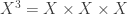 is hereditarily normal, then
 is a maximal almost disjoint family of subsets of
  .
. is an infinite subset of
  be a limit point of
  . The candidate for a non-normal subspace of
 is an open subspace of
 for each
  . Furthermore each
  . Since
  such that
  . Then
  and
and  .
.  and
and  such that
  and
and  . With
  , there exists some
  . First,
  . Since
  . Thus
 is said to be the diagonal of the space
  be an uncountable cardinal. Let
  be the Cartesian product of
  as a closed subspace. However, there are dense subspaces of
  are normal. For example, the
  -product of
  where
where  be a topological space. A collection
  of subsets of
  and for each open
  with
with  , there exists some
  such that
  . A countable network is a network that has only countably many elements. The property of having a countable network is a very strong property, e.g., having all the properties listed above. For a basic discussion of this property, see
  and for any open interval
  in the real line with rational endpoints, consider the following set:
![[B,(a,b)]=\left\{f \in C(X): f(B) \subset (a,b) \right\}](https://s0.wp.com/latex.php?latex=%5BB%2C%28a%2Cb%29%5D%3D%5Cleft%5C%7Bf+%5Cin+C%28X%29%3A+f%28B%29+%5Csubset+%28a%2Cb%29+%5Cright%5C%7D&bg=ffffff&fg=333333&s=0&c=20201002)
![[B,(a,b)]](https://s0.wp.com/latex.php?latex=%5BB%2C%28a%2Cb%29%5D&bg=ffffff&fg=333333&s=0&c=20201002) . Let
. Let  where
where ![O=\bigcap_{x \in F} [x,O_x]](https://s0.wp.com/latex.php?latex=O%3D%5Cbigcap_%7Bx+%5Cin+F%7D+%5Bx%2CO_x%5D&bg=ffffff&fg=333333&s=0&c=20201002) is a basic open set in
is a basic open set in  is an open interval with rational endpoints. For each point
  , choose
  with
with  such that
  . Clearly
 ![f \in \bigcap_{x \in F} \ [B_x,O_x]](https://s0.wp.com/latex.php?latex=f+%5Cin+%5Cbigcap_%7Bx+%5Cin+F%7D+%5C+%5BB_x%2CO_x%5D&bg=ffffff&fg=333333&s=0&c=20201002) . It follows that
. It follows that ![\bigcap_{x \in F} \ [B_x,O_x] \subset O](https://s0.wp.com/latex.php?latex=%5Cbigcap_%7Bx+%5Cin+F%7D+%5C+%5BB_x%2CO_x%5D+%5Csubset+O&bg=ffffff&fg=333333&s=0&c=20201002) .
. ,
, ![C_p([0,1])](https://s0.wp.com/latex.php?latex=C_p%28%5B0%2C1%5D%29&bg=ffffff&fg=333333&s=0&c=20201002) and
and  . All three can be considered subspaces of the product space
  where
where  is the cardinality of the continuum. This is true for any separable metrizable
  . The product space
  continuum many copies of the real lines, hence can be regarded as a subspace of
  of the separable metric spaces
  is a dense and normal subspace of the product space
  . The normal space
 and for each positive integer
  be the open arc in
  (in the Euclidean topology on
  where
where
 ).
).

 where the topology is generated by a base consisting the half open intervals of the form
  . The Sorgenfrey plane is the square
  of open covers of
  , and for each open subset
  , there exists one cover
  satisfying the condition that for any open set
  ,
,  . When
  increases. In fact, this is how a development is defined for a metric space, where
  . Thus metric spaces are developable. There are plenty of non-metrizable Moore space. One example is the
  . Then
  is a countable base for
  -locally finite base for
  -space and for every discrete collection
  of closed sets in
  of open subsets of
  . For a proof of Bing’s metrization theorem, see page 329 of [1].
 denote the real number line and
  denote the set of all irrational numbers. The irrational numbers and the set
  where each
  has the discrete topology. We will also denote the product space
  . We have the following theorem.
 such that
  . We divide the real line into countably many non-overlapping intervals. Specifically, let
 ![A_0=[0,1]](https://s0.wp.com/latex.php?latex=A_0%3D%5B0%2C1%5D&bg=ffffff&fg=333333&s=0&c=20201002) ,
, ![A_1=[-1,0]](https://s0.wp.com/latex.php?latex=A_1%3D%5B-1%2C0%5D&bg=ffffff&fg=333333&s=0&c=20201002) ,
, ![A_2=[1,2]](https://s0.wp.com/latex.php?latex=A_2%3D%5B1%2C2%5D&bg=ffffff&fg=333333&s=0&c=20201002) , etc (see the following figure).
, etc (see the following figure).
 by
by  and denote the right endpoint by
  .
. of rational numbers converging to the right endpoint
 ![A_{i,0}=[L_i,x_{i,0}]](https://s0.wp.com/latex.php?latex=A_%7Bi%2C0%7D%3D%5BL_i%2Cx_%7Bi%2C0%7D%5D&bg=ffffff&fg=333333&s=0&c=20201002) ,
, ![A_{i,1}=[x_{i,0},x_{i,1}]](https://s0.wp.com/latex.php?latex=A_%7Bi%2C1%7D%3D%5Bx_%7Bi%2C0%7D%2Cx_%7Bi%2C1%7D%5D&bg=ffffff&fg=333333&s=0&c=20201002) ,
, ![A_{i,2}=[x_{i,1},x_{i,2}]](https://s0.wp.com/latex.php?latex=A_%7Bi%2C2%7D%3D%5Bx_%7Bi%2C1%7D%2Cx_%7Bi%2C2%7D%5D&bg=ffffff&fg=333333&s=0&c=20201002) , etc (see the following figure).
, etc (see the following figure).
 . One is that we make sure the rational number
  is chosen as an endpoint of some interval in Step 1. The second is that the length of each
  is less than
  .
. and
and  , respectively. We choose a sequence
  of rational numbers converging to the left endpoint
 ![A_{i,j,0}=[x_{i,j,0},R_{i,j}]](https://s0.wp.com/latex.php?latex=A_%7Bi%2Cj%2C0%7D%3D%5Bx_%7Bi%2Cj%2C0%7D%2CR_%7Bi%2Cj%7D%5D&bg=ffffff&fg=333333&s=0&c=20201002) ,
, ![A_{i,j,1}=[x_{i,j,1},x_{i,j,0}]](https://s0.wp.com/latex.php?latex=A_%7Bi%2Cj%2C1%7D%3D%5Bx_%7Bi%2Cj%2C1%7D%2Cx_%7Bi%2Cj%2C0%7D%5D&bg=ffffff&fg=333333&s=0&c=20201002) ,
, ![A_{i,j,2}=[x_{i,j,2},x_{i,j,1}]](https://s0.wp.com/latex.php?latex=A_%7Bi%2Cj%2C2%7D%3D%5Bx_%7Bi%2Cj%2C2%7D%2Cx_%7Bi%2Cj%2C1%7D%5D&bg=ffffff&fg=333333&s=0&c=20201002) , etc (see the following figure).
, etc (see the following figure).
 . One is that we make sure the rational number
  is chosen as an endpoint of some interval in Step 2. The second is that the length of each
  is less than
  .
. are rational numbers and we make sure that all the rational numbers are used as endpoints. We also make sure that the intervals from the successive steps are nested closed intervals with lengths
  . The consequence of this point is that the nested decreasing closed intervals will collapse to one single point (since the real line is a complete metric space) and this single point must be an irrational number (since all the rational numbers are used up as endpoints of the nested closed intervals).
 where
where  is an even integer, we make the endpoints of the new intervals converge to the left. This manipulation is to ensure that the nested closed intervals will never share the same endpoint from one step all the way to the end of the process.
 , then
  and in fact has only one point that is an irrational number.
  , we can locate inductively a sequence of intervals,
  , containing the point
  is a local base at the point
  . One the other hand, each
  has a natural counterpart in a basic open set in the product space, namely the following set:
 . In contrast to this example, S. Willard has shown that, if
 ![[0,1]^{\mathcal{K}}](https://s0.wp.com/latex.php?latex=%5B0%2C1%5D%5E%7B%5Cmathcal%7BK%7D%7D&bg=ffffff&fg=333333&s=0&c=20201002) where
where  is any uncountable cardinal.
 is clear. To see
  , let
, let  and let
  be a collection of open subsets of
  ,
,  for some
  . Then
  is Lindelof. We can find countably many sets in
  be an open subset. For each
  be open such that
  (this comes from the fact that
  equals
  is Lindelof and
  is paracompact, but
  , choose open
  such that
  and
and  be the union of the finitely many
  . Then
  belongs to one of the countably many
  compact space, then
  is Lindelof by Theorem 4. Furthermore,
  be either the closed unit interval
 ![\mathbb{I}=[0,1]](https://s0.wp.com/latex.php?latex=%5Cmathbb%7BI%7D%3D%5B0%2C1%5D&bg=ffffff&fg=333333&s=-1&c=20201002) or
or ![[0,\omega]=\omega+1](https://s0.wp.com/latex.php?latex=%5B0%2C%5Comega%5D%3D%5Comega%2B1&bg=ffffff&fg=333333&s=-1&c=20201002) . Let
. Let  be any one of the following spaces:
![X=[0,\omega_1]=\omega_1+1](https://s0.wp.com/latex.php?latex=X%3D%5B0%2C%5Comega_1%5D%3D%5Comega_1%2B1&bg=ffffff&fg=333333&s=-1&c=20201002) ,
, ,
, Michael Line,
 is normal in all four cases. The
  be a closed set that is not a
  set. Let
  be an infinite set with an accumulation point
  .
. is not normal. To this end, let
  and
and  . The sets
  and
and  are disjoint closed subspaces of the open subspace
  . Suppose we have disjoint open sets
  and
and  such that
  and
and  .
.  , let
, let  . Each
  is open and
  . Thus
  . Let
. Let  . Then
  . This means
  . If
. If  , then
  (which is impossible). So we have
  , indicating that
  is a
is a 