We discuss the completeness of the real line. With respect to the real line, completeness refers to the fact that the real line has no holes or gaps. There are many ways to state what it means for the real line to be complete. In this post, we state it using the least upper bound property. Then we show that this property is equivalent to a host of other statements. This discussion will be useful for subsequent posts where we discuss compactness and other properties of the real line.
This is a post on introductory topology. Concepts discussed here are basic notions found in beginning topology courses and elementary analysis courses. For the readers who are taking math courses that transition their math career from calculation to proving of theorems, we encourage such readers to think about the concepts and theorems discussed here before reading the proofs.
Let  . By an upper bound of the set
  , we mean a real number number
  such that
  for all
  . If a set has an upper bound, we say that it is bounded above. Similarly, a lower bound of the set is a real number
  such that
  for all . If a set has a lower bound, then we say it is bounded below. If a set is both bounded above and bounded below, it is said to be bounded.
Suppose is bounded above. By a least upper bound of the set , we mean a real number  that is the smallest among all the upper bounds of , that is, the number is itself an upper bound of and for each upper bound of , we have
  . It turns out that if a set has a least upper bound, then it is unique. Suppose and
  are both least upper bounds of . Then we have
  and
and  . This imples
  .
.
Similarly, the number  is the greatest lower bound of the set if the number is a lower bound of and for each lower bound of , we have
  . As with the least upper bound, if a set has a greatest lower bound, it has only one greatest lower bound. The following is the statement of the least upper bound property:
The Least Upper Bound Property. Every subset of the real line that is bounded above has a least upper bound.
In the discussion about the real line in this post and in subsequent posts, we will take the least upper bound property as a given. In the remainder of this post, we show that this property is equivalent to several other statements about the real line. Thus we could have taken any one of those statements as a given. We also have a statement that can be called the greatest lower bound property: every subset of the real line that is bounded below has a greatest lower bound. This statement is also equivalent to the least upper bound property.
For the definition of open intervals, open sets and closed sets, see the previous post The Euclidean topology of the real line (2). We have some more definitions.
Definitions
- Let . Let
 . The point
  is a limit point of if every open set containing contains a point of different from .
- Let
 be the set of all positive integers. A sequence of real numbers is a function
  . We usually express
  as
as  and the function
  is expressed as
  or
or  .
.
- Given a sequence of real numbers , consider an infinite subset
 . If we only consider terms of the sequence where the subscript
  , then it is called a subsequence of . The notation is
  .
.
- A sequence converges if there is a number such that for every open interval
 containing , there is a positive integer
  such that
  for all
  . The point is said to be the limit of . We use the notation
  or
or  .
.
- A sequence is said to be a Cauchy sequence if for each
 , there is a positive integer such that
  for all
  .
.
- A sequence is said to be bounded if the set of the terms of the sequence
 is a bounded set, or equivalently there is a positive number
  such that for each term we have
  .
.
- A sequence is said to be nondecreasing if
 for each
  . For such a sequence, we have
  .
.
- A sequence is said to be nonincreasing if
 for each . For such a sequence, we have
  .
.
- A sequence is said to be monotonic if it is either nondecreasing or nonincreasing.
One of the properties that is equivalent to the least upper bound property is the nested interval property. It is stated as follows:
The Nested Interval Property. Suppose that for each positive interger  we have closed intervals
 ![I_n=[a_n,b_n]](https://s0.wp.com/latex.php?latex=I_n%3D%5Ba_n%2Cb_n%5D&bg=ffffff&fg=333333&s=0&c=20201002) such that
such that
![\displaystyle [a_1,b_1] \supset [a_2,b_2] \supset [a_3,b_3] \supset \cdots](https://s0.wp.com/latex.php?latex=%5Cdisplaystyle+%5Ba_1%2Cb_1%5D+%5Csupset+%5Ba_2%2Cb_2%5D+%5Csupset+%5Ba_3%2Cb_3%5D+%5Csupset+%5Ccdots&bg=ffffff&fg=333333&s=0&c=20201002)
and  .
.
Then the intersection of the intervals  has only one point, i.e.
 ![\bigcap \limits_{n=1}^{\infty} [a_n,b_n]=\left\{x\right\}](https://s0.wp.com/latex.php?latex=%5Cbigcap+%5Climits_%7Bn%3D1%7D%5E%7B%5Cinfty%7D+%5Ba_n%2Cb_n%5D%3D%5Cleft%5C%7Bx%5Cright%5C%7D&bg=ffffff&fg=333333&s=0&c=20201002) .
.
We incorporate some observations about sequences into a lemma, which is used in proving the main theorem below.
Lemma
- If a sequence
 of real numbers converges, then the limit is unique.
- If a sequence of real numbers converges, then the sequence is a Cauchy sequence.
- If is a Cauchy sequence of real numbers, then it is bounded.
- If a sequence of real numbers converges, then the sequence is bounded.
- If the real number is a limit point of the set , then there is a sequence of points of such that converges to .
Proof
 Note that if a sequence converges to a point , then every open interval containing would contain all but finitely many terms in the sequence. Point in the lemma stems from the fact that every pair of distinct numbers in the real line are contained in two disjoint open intervals. For
  , we have disjoint open intervals
  and
and  where
where  . If both
  and are limits of the same sequence, then each of these two disjoint open intervals would contain all but finitely many terms in the sequence, which is impossible.
 Let be a convergent sequence with as a limit. For each , we have such that
  for all . Thus for all , we have:

The above shows that the sequence is a Cauchy sequence.
 Let be a Cauchy sequence. For
  , there is some positive integer such that for all , we have
  . Let be the maximum of the following real numbers:

Then for each term  in the sequence we have
  . Furthermore, we have:

Thus  is an upper bound of the cauchy sequence in question.
 This follows from and .
 Let be a limit point of the set . For each positive integer
  , let
, let  such that
  . Then
  .
.
Theorem
The following statements are equivalent:
- The least upper bound property.
- Every bounded montonic sequence of real numbers converges.
- The nested interval property.
- (Bolzano-Weierstrass Theorem) Every infinite set of real numbers that is also bounded has a limit point.
- Every bounded sequence of real numbers has a subsequence that converges.
- Every Cauchy sequence of real numbers converges.
Remark
In some texts such as ![[1]](https://s0.wp.com/latex.php?latex=%5B1%5D&bg=ffffff&fg=333333&s=0&c=20201002) , completeness is defined in terms of Cauchy sequences (condition
, completeness is defined in terms of Cauchy sequences (condition  ). In a metric space, a Cauchy sequence is one where the distances of the successive terms diminishes to zero. Any space with a metric such that every Cauchy sequence converges is said to be a complete metric space. Thus the real line with the Euclidean metric is an example of a complete metric space.
In some texts, the nested interval property is taken as the definition of completeness. In a general metric space, the nested intervals are taken to be closed and bounded sets (bounded by the metric in question) with diameters  .
.
The least upper bound property is based on an order relation and is not applicable to metric spaces in general. Conditions  do not hold in metric spaces in general but hold in Euclidean spaces.
Proof
We establish the equivalences by proving  ,
,  ,
,  ,
,  ,
,  ,
,  and
and  .
.
We show that every bounded nondecreasing sequence of real numbers converges. For the proof that every bounded nonincreasing sequence of real numbers converges, use a similar proof by working with the greatest lower bound. Suppose that the sequence is nondecreasing and bounded. Let be an upper bound of the set  . By the least upper bound property, the set has a least upper bound . We have the following:

We claim that the number is the limit of the sequence . Let be an open interval containing , i.e,  . There must be some term
  of the sequence such that
  . Otherwise,
  would be an upper bound, which is impossible since is the least upper bound. Since the sequence is nondecreasing, we have
  for all
  . Thus is established.
Suppose we have a sequence of nested intervals ![[a_n,b_n]](https://s0.wp.com/latex.php?latex=%5Ba_n%2Cb_n%5D&bg=ffffff&fg=333333&s=0&c=20201002) such that the widths of the intervals
such that the widths of the intervals  . The sequence
  is nondecreasing and has an upper bound (e.g.
  ). By , this sequence converges, say to the limit . On the other hand, the sequence
  is nonincreasing and has an lower bound (e.g.
  ). Thus this sequence converges, say to the limit
  .
.
Note that ![[a,b] \subset [a_n,b_n]](https://s0.wp.com/latex.php?latex=%5Ba%2Cb%5D+%5Csubset+%5Ba_n%2Cb_n%5D&bg=ffffff&fg=333333&s=0&c=20201002) for each . Since ,
for each . Since ,  .
.
Suppose is an infinite set and is bounded. We produce a limit point by the approach of “divide and conquer”. Suppose that ![A \subset [a,b]](https://s0.wp.com/latex.php?latex=A+%5Csubset+%5Ba%2Cb%5D&bg=ffffff&fg=333333&s=0&c=20201002) . Let
. Let  and
and  . Divide this interval into two equal halves,
 ![[a_1,m]](https://s0.wp.com/latex.php?latex=%5Ba_1%2Cm%5D&bg=ffffff&fg=333333&s=0&c=20201002) and
and ![[m,b_1]](https://s0.wp.com/latex.php?latex=%5Bm%2Cb_1%5D&bg=ffffff&fg=333333&s=0&c=20201002) where
where  . Since is infinite, one of these two halves has to contain infinitely many points of . Otherwise, is a finite set. Pick a half that has infinitely many points of and let
  be the left endpoint of this interval and
  be the right endpoint.
Continue this process inductively. Suppose has been chosen. Then we divide it into ![[a_n,m]](https://s0.wp.com/latex.php?latex=%5Ba_n%2Cm%5D&bg=ffffff&fg=333333&s=0&c=20201002) and
and ![[m,b_n]](https://s0.wp.com/latex.php?latex=%5Bm%2Cb_n%5D&bg=ffffff&fg=333333&s=0&c=20201002) where
where  . Pick a half that has infinitely many points of and let
  be the left endpoint and
  be the right endpoint. Then we have a nested sequence of decreasing intervals. Since we keep dividing each stage into halves, the lengths of the intervals
  approaches
  . By the nested interval property, there is only one point in the intersection of the intervals.
The point is a limit point of . To see this, let  be an open interval containing . Then for some sufficiently large we have
 ![[a_n,b_n] \subset (s,t)](https://s0.wp.com/latex.php?latex=%5Ba_n%2Cb_n%5D+%5Csubset+%28s%2Ct%29&bg=ffffff&fg=333333&s=0&c=20201002) . Then the open interval contains infinitely many points of .
. Then the open interval contains infinitely many points of .
Suppose is a bounded sequence of real numbers. We aim to produce a subsequence that converges. Let be the set of all terms in the sequence. The set is expressed as the following:

Suppose is a finite set. Then starting at some integer ,  . The sequence
  is a subsequence that is a constant sequence (thus converges). Suppose is an infinite set. By , has a limit point. Let be one limit point of . By in the lemma, there is a sequence of points from converging to . This sequence would be a subsequence of .
By the lemma, any Cauchy sequence of real numbers is bounded. Let be a Cauchy sequence of real numbers. By , there is a subsequence  that converges. Let be the limit of the subsequence. Note that is also the limit of the original sequence .
Let be a sequence of intervals satisfying the nested interval property. Then is a Cauchy sequence, which converges, say to the point . Then is the lone point that belongs to each .
Suppose that is bounded above. Let  be the set of all upper bounds of . Note that for each , is a lower bound of . Pick and
  . Let
. Let  and
and  . If there are only finitely many point of in between and , then the smallest points of would be the least upper bound of and we are done. So assume that
 ![[a_1,b_1]](https://s0.wp.com/latex.php?latex=%5Ba_1%2Cb_1%5D&bg=ffffff&fg=333333&s=0&c=20201002) contains infinitely many points of (i.e. infinitely many upper bounds of ).
contains infinitely many points of (i.e. infinitely many upper bounds of ).
Consider and where . If the left interval contains upper bounds of , we assume that that it has infinitely many of them (otherwise, the minimum would be the least upper bound and we are done). Choose one of these intervals that contains infinitely many points of . If both intervals contain infinitely many points of , we choose the leftmost one. Then we let be the left endpoint of the chosen interval and be the right endpoint of the interval. We observe that to the left of , there are no upper bounds of (points of ).
Continue this process inductively, making sure that in each step we divide the previous interval into two equal halves. If the left interval contains upper bounds of , we assume that it has infinitely many of them (otherwise, we stop at this inductive step). We choose the first half interval that contains infinitely many upper bounds of and denote it by ![[a_{n+1},b_{n+1}]](https://s0.wp.com/latex.php?latex=%5Ba_%7Bn%2B1%7D%2Cb_%7Bn%2B1%7D%5D&bg=ffffff&fg=333333&s=0&c=20201002) . Observe that to the left of , there are no upper bounds of .
. Observe that to the left of , there are no upper bounds of .
As indicated in the induction step, if we can stop at any one of the step, we would have a least upper bound of and we are done. Otherwise, we have a nested sequence of intervals such that the widths of the intervals . Then the intervals have exactly one point in the intersection.
We claim that is the desired least upper bound of . First of all, there is no upper bounds of to the left of . This stems from the observation that no upper bounds of can be found at the left side of each  and the fact that
  converges to . Thus if is an upper bound of , then is the least upper bound. Note that is a limit point of since every interval contains infinitely many points of . If is not an upper bound of , then there is some point
  of such that
  . Then the interval
  contains no points of (upper bounds of ). This constradicts the fact that is a limit point of . So must be an upper bound of . This establishes the least upper bound property.
Reference
- Rudin, W., Principles of Mathematical Analysis, Third Edition, 1976, McGraw-Hill, New York.

 , we construct a Cantor set within
 ![[a,b]](https://s0.wp.com/latex.php?latex=%5Ba%2Cb%5D&bg=ffffff&fg=333333&s=0&c=20201002) .
.![x \in [a,b]](https://s0.wp.com/latex.php?latex=x+%5Cin+%5Ba%2Cb%5D&bg=ffffff&fg=333333&s=0&c=20201002) such that
such that  .
. . The point
  contains a point of
  contains a point of
  is an uncountable set. Then
  contains a two-sided limit point.
 is a nonempty perfect set that satisfies Case 2 indicated above. Suppose that for the closed interval
  ,
, ,
, such that:
 ,
, is a left-sided limit point of
  is a right-sided limit point of
  such that
  . Then we can find an open interval
  such that
  and
and  and
and  .
. . By the least upper bound property,
  has a least upper bound
 ![W_2=(d,b] \cap E](https://s0.wp.com/latex.php?latex=W_2%3D%28d%2Cb%5D+%5Ccap+E&bg=ffffff&fg=333333&s=0&c=20201002) . By the greatest lower bound property,
. By the greatest lower bound property,  has a greatest lower bound
![[s,t]](https://s0.wp.com/latex.php?latex=%5Bs%2Ct%5D&bg=ffffff&fg=333333&s=0&c=20201002) such that the left endpoint
such that the left endpoint  is a right-sided limit point of
  is a left-sided limit points of
  such that:
 contains points of
  and
and  are two-sided limit points of
  .
.![E_1=[s,t] \cap E](https://s0.wp.com/latex.php?latex=E_1%3D%5Bs%2Ct%5D+%5Ccap+E&bg=ffffff&fg=333333&s=0&c=20201002) is a nonempty perfect set. Thus
is a nonempty perfect set. Thus  is uncountable. So pick
  such that
  and
and  . Since
  and
and  such that
  ,
,  and both
 ![K_0=[p_0,q_0]](https://s0.wp.com/latex.php?latex=K_0%3D%5Bp_0%2Cq_0%5D&bg=ffffff&fg=333333&s=0&c=20201002) and
and ![K_1=[p_1,q_1]](https://s0.wp.com/latex.php?latex=K_1%3D%5Bp_1%2Cq_1%5D&bg=ffffff&fg=333333&s=0&c=20201002) such that
such that![K_0 \subset [a,b]](https://s0.wp.com/latex.php?latex=K_0+%5Csubset+%5Ba%2Cb%5D&bg=ffffff&fg=333333&s=0&c=20201002) and
and ![K_1 \subset [a,b]](https://s0.wp.com/latex.php?latex=K_1+%5Csubset+%5Ba%2Cb%5D&bg=ffffff&fg=333333&s=0&c=20201002) ,
, and
and  are less then
  ,
,![[a,a^*]](https://s0.wp.com/latex.php?latex=%5Ba%2Ca%5E%2A%5D&bg=ffffff&fg=333333&s=0&c=20201002) and
and ![[b^*,b]](https://s0.wp.com/latex.php?latex=%5Bb%5E%2A%2Cb%5D&bg=ffffff&fg=333333&s=0&c=20201002) . Each of these two subintervals contains points of the perfect set
. Each of these two subintervals contains points of the perfect set  and is thus less than
  and is thus less than
  and
and  perfect sets and compact sets.
  is a nonempty perfect set that satisfies Case 2. Pick two two-sided limit
  and
and  of
of  and
and  as a result of applying Lemma 4. Let
  .
. and obtain closed intervals
  ,
,  . Likewise we apply Lemma 4 on the closed interval
  and obtain closed intervals
  ,
,  . Let
. Let  .
. . The set
  is a Cantor set and has all the properties discussed in the posts labled #6 and #7 lised at the end of this post.
  . For any countably infinite sequence
  of zeros and ones, let
  be the first
  . Then
  for some countably infinite sequence
  . Thus
  .
. of all integers (positive, negative and zero) is a closed set as well as a discrete set. It is closed because the complement is an open set. It is discrete since no point of
  Every uncountable subset has a limit point.
 is a discrete set, as is the set
  is not a closed set. It turns out that in the real line, only countable sets can be discrete. Equivalently, the real line satisfies the following property:
 Every uncountable subset contains one of its limit points.
 and
and  are intimately tied to the Lindelof property. Specifically, both
  of subsets of
  also covers
  is said to be a subcover of
  be uncountable such that
  such that
  and
and 
 is an open set relative to
  has the Lindelof property, i.e.
  , we have
  . The point
  . The point
  , choose a rational number
  such that
  contains no point of
  such that
  for uncountably many
 . This is possible since
  for all
  and
and  such that
  . Otherwise,
  contains infinitely many points of
  is supposed to contain no points of
  are compact subsets of the real line such that
 .
. .
.
 such that
  . Next, pick an open interval
  such that
  and
and  and
and  .
. stage where
  , pick an open interval
  such that
  and
and  and
and  . Since
  . Note that
  is a compact set since
  is compact. By the lemma, the intersection of the
  . In this construction, we remove the middle
  open interval of
 ![[0,1]](https://s0.wp.com/latex.php?latex=%5B0%2C1%5D&bg=ffffff&fg=333333&s=0&c=20201002) . This removed open interval has length
. This removed open interval has length  and the remaining set has length
  .
.  . Thus, the length of the remaining set is
  .
. . Then the remaining set has length:
  .
.
 , we have the middle third Cantor set that is constructed in the previous post
  . For the illustration here, we use
  where
where  . Note that
  .
. , making the left over piece of length
  , we remove the middle
  open interval of
  , in each of the remaining two closed intervals, we remove the middle part such that the two removed open intervals have equal length and the combined length of
  .
. , the four removed open intervals are of equal length and with a combined total length of
  .
. since
since  . Yet the points remained have the same cardinality as the unit interval
  where
where![A_0=[0,1]](https://s0.wp.com/latex.php?latex=A_0%3D%5B0%2C1%5D&bg=ffffff&fg=333333&s=0&c=20201002)

 , where
  and
and  are obtained by removing the middle third of the closed interval
  where
where  and
and  agree on the first
  many coordinates if
  . The
. The  or
or  . Say
. Say  or
or  . Say,
  or
or  . Say,
 , which is a sequence of countably infinite many zeros and ones such that the first
  in the above paragraph is a bijection between the Cantor set
  , the set of all countably infinite sequences of zeros and ones. If
  , we let
  .
. form a local base at
  , there is some integer
  .
. be the set of endpoints of the closed intervals
  .
.

![[0,1]-C](https://s0.wp.com/latex.php?latex=%5B0%2C1%5D-C&bg=ffffff&fg=333333&s=0&c=20201002) , the complement of
, the complement of  where each
 ![y \in [0,1]](https://s0.wp.com/latex.php?latex=y+%5Cin+%5B0%2C1%5D&bg=ffffff&fg=333333&s=0&c=20201002) . If
. If ![y \in [0,1]-C](https://s0.wp.com/latex.php?latex=y+%5Cin+%5B0%2C1%5D-C&bg=ffffff&fg=333333&s=0&c=20201002) , then we are done. So suppose
, then we are done. So suppose ![(a,b) \cap ([0,1]-C) \ne \phi](https://s0.wp.com/latex.php?latex=%28a%2Cb%29+%5Ccap+%28%5B0%2C1%5D-C%29+%5Cne+%5Cphi&bg=ffffff&fg=333333&s=0&c=20201002) .
.  . By 3,
  such that
  . To say that
  . But the Cantor set
  .
.  and
and  , both containing points of
  . A set
 ![C=([0,0.5) \cap C) \cup (0.5,1] \cap C)](https://s0.wp.com/latex.php?latex=C%3D%28%5B0%2C0.5%29+%5Ccap+C%29+%5Ccup+%280.5%2C1%5D+%5Ccap+C%29&bg=ffffff&fg=333333&s=0&c=20201002) .
. with
with  where
where  such that
  . Then we have:
![\displaystyle A=([0,t) \cap A) \cup ((t,1] \cap A)](https://s0.wp.com/latex.php?latex=%5Cdisplaystyle+A%3D%28%5B0%2Ct%29+%5Ccap+A%29+%5Ccup+%28%28t%2C1%5D+%5Ccap+A%29&bg=ffffff&fg=333333&s=0&c=20201002)
 be the set of all sequences zeros and ones of length
  ,
,  ,
,  and so on. Each
  sequences. For each
  , we can tag on a
  . For example, for
  , both
  .
. from
from  . Label the remaining two intervals by
 ![B_0=[0,\frac{1}{3}]](https://s0.wp.com/latex.php?latex=B_0%3D%5B0%2C%5Cfrac%7B1%7D%7B3%7D%5D&bg=ffffff&fg=333333&s=0&c=20201002) and
and ![B_1=[\frac{2}{3},1]](https://s0.wp.com/latex.php?latex=B_1%3D%5B%5Cfrac%7B2%7D%7B3%7D%2C1%5D&bg=ffffff&fg=333333&s=0&c=20201002) . Let
. Let  , remove the middle third of
 ![B_{00}=[0,\frac{1}{9}]](https://s0.wp.com/latex.php?latex=B_%7B00%7D%3D%5B0%2C%5Cfrac%7B1%7D%7B9%7D%5D&bg=ffffff&fg=333333&s=0&c=20201002) and
and ![B_{01}=[\frac{2}{9},\frac{1}{3}]](https://s0.wp.com/latex.php?latex=B_%7B01%7D%3D%5B%5Cfrac%7B2%7D%7B9%7D%2C%5Cfrac%7B1%7D%7B3%7D%5D&bg=ffffff&fg=333333&s=0&c=20201002) . For
. For  , remove the meddle third of
 ![B_{10}=[\frac{2}{3},\frac{7}{9}]](https://s0.wp.com/latex.php?latex=B_%7B10%7D%3D%5B%5Cfrac%7B2%7D%7B3%7D%2C%5Cfrac%7B7%7D%7B9%7D%5D&bg=ffffff&fg=333333&s=0&c=20201002) and
and ![B_{11}=[\frac{8}{9},1]](https://s0.wp.com/latex.php?latex=B_%7B11%7D%3D%5B%5Cfrac%7B8%7D%7B9%7D%2C1%5D&bg=ffffff&fg=333333&s=0&c=20201002) . Let
. Let  is
is  .
. .
. has been defined for each
  .
. .
. . For each closed interval
  and
and  where each has length
  . Let
. Let  be defined as:
 . This is a nonempty set subset of the unit interval. The point
  since
since  . Being the union of finitely many closed intervals, each
  is a one-to-one function if for
  ,
,  , that is, distinct elements of the domain are mapped to distinct elements of the range. A function
  , i.e. every point in the set
  . For example, the set of all rational numbers has the same cardinality as the integers since we can define a bijection between the two sets. More informally, we can put the rational numbers in an exhaustive list indexed by the integers. When a set has the same cadinality as the set of real numbers, we say that the set has cardinality continuum.
 . Obviously when
  , we have
  , we have
  , we have
  be the set of all nonnegative integers. Let
  be the set of subsets of
  . The cardinality of the Cantor set follows from the following relationship:
 is clear since the Cantor set is a subset of the real line. The following claims establish the relationship.
 . At the next stage, the point
  .
. agree on the first
  such that
  .
. . This mapping is one-to-one. For
  where
where  . Let
. Let  in stage
  . However,
  and
and  . As a result,
  and
and  disagree at the
  .
. .
. 
 ,
,  such that the
  is:
is:
 is a one-to-one map and that
  .
. 
 be the set of all rational numbers. Since
  , we have
  . We now define a one-to-one map
  .
. , let
, let  . It is clear that
  for
for  where
where 


 is either 0 or 1 and is the result of the
  toss in the
  sequence in the list. We consider the terms in the diagonal
  and so on. Then for each
  , define
  as the following:
 is an outcome of tossing infinitely many coins that is not on the listing. Thus, in attempting to make an exhaustive listing, we can always come up with another outcome that is not on the listing. This means the set of all possible sequences of 0’s and 1’s is an uncountable set. In the next post, we will show that it is the same size as the real numbers. These sequences of 0’s and 1’s are important in the construction of the Cantor set.
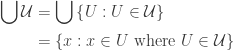
 denotes the union of all sets in
  .
.
 , that is, every point in
  .
. is an open cover of
  is compact since any open interval containing
  .
. . Let
. Let 
 . The singleton set
  is surely not an open subset of the whole real line. However, it is open relative to the space
  . The property of being closed sets is also relative. The interval
  is a closed set relative to the space
  Let
Let 
 has a finite subcollection that is also an open cover. The following lists out this finite subcollection:
 and covers
  Let
Let  where
where 
 is an open cover of
  such that
  is a cover of
 is a cover of
  is a collection of compact subsets of
  .
. . Then the following is an open cover of the compact set
 such that
  covers
  , contradicting that the collection
  of
of  . The set
  .
.
 . For each
  , there is an open set
  such that
  . Furthermore, there is an open interval
  such that the endpoints are rational numbers and
  . Each
  is associated with at least one
  . Thus for each
  such that
  . Then
  is the desired subcollection.
  This follows from definition and lemma 3. See the remark right below lemma 3.
 Suppose that
  contains
  is an open cover of
  Suppose that
  Suppose that
  in the main theorem in the previous post (
 such that
  . The set
  is an infinite set. Note that
  Suppose that
  such that no finite subset of
  .
. has a convergent subsequence
  where
where  is an infinite subset of
 ![\left\{[a_n,b_n]\right\}](https://s0.wp.com/latex.php?latex=%5Cleft%5C%7B%5Ba_n%2Cb_n%5D%5Cright%5C%7D&bg=ffffff&fg=333333&s=0&c=20201002) such that
such that ![\displaystyle [a_1,b_1] \supset [a_2,b_2] \supset \cdots](https://s0.wp.com/latex.php?latex=%5Cdisplaystyle+%5Ba_1%2Cb_1%5D+%5Csupset+%5Ba_2%2Cb_2%5D+%5Csupset+%5Ccdots&bg=ffffff&fg=333333&s=0&c=20201002) .
.![\bigcap \limits_{n=1}^{\infty} [a_n,b_n] \ne \phi](https://s0.wp.com/latex.php?latex=%5Cbigcap+%5Climits_%7Bn%3D1%7D%5E%7B%5Cinfty%7D+%5Ba_n%2Cb_n%5D+%5Cne+%5Cphi&bg=ffffff&fg=333333&s=0&c=20201002) .
. is the Heine-Borel theorem. Theorem 5 completely characterizes the compact subsets of the real line, namely the subsets that are closed and bounded (closed relative to the real line). By the theorem, closed intervals
  .
.