A little corner in the world of set-theoretic topology

Posted on October 15, 2018 by Dan Ma

This post puts a spot light on a little corner in the world of set-theoretic topology. There lies in this corner a simple topological statement that opens a door to the esoteric world of independence results. In this post, we give a proof of this basic fact and discuss its ramifications. This basic result is an excellent entry point to the study of S and L spaces.

The following paragraph is found in the paper called Gently killing S-spaces by Todd Eisworth, Peter Nyikos and Saharon Shelah [1]. The basic fact in question is highlighted in blue.

A simultaneous generalization of hereditarily separable and hereditarily Lindelof spaces is the class of spaces of countable spread – those spaces in which every discrete subspace is countable. One of the basic facts in this little corner of set-theoretic topology is that if a regular space of countable spread is not hereditarily separable, it contains an L-space, and if it is not hereditarily Lindelof, it contains an S-space. [1]

The same basic fact is also mentioned in the paper called The spread of regular spaces by Judith Roitman [2].

It is also well known that a regular space of countable spread which is not hereditarily separable contains an L-space and a regular space of countable spread which is not hereditarily Lindelof contains an S-space. Thus an absolute example of a space satisfying (Statement) A would contain a proof of the existence of S and L space – a consummation which some may devoutly wish, but which this paper does not attempt. [2]

Statement A in [2] is: There exists a 0-dimensional Hausdorff space of countable spread that is not the union of a hereditarily separable and a hereditarily Lindelof space. Statement A would mean the existence of a regular space of countable spread that is not hereditarily separable and that is also not hereditarily Lindelof. By the well known fact just mentioned, statement A would imply the existence of a space that is simultaneously an S-space and an L-space!

Let’s unpack the preceding section. First some basic definitions. A space $X$ is of countable spread (has countable spread) if every discrete subspace of $X$ is countable. A space $X$ is hereditarily separable if every subspace of $X$ is separable. A space $X$ is hereditarily Lindelof if every subspace of $X$ is Lindelof. A space is an S-space if it is hereditarily separable but not Lindelof. A space is an L-space if it is hereditarily Lindelof but not separable. See [3] for a basic discussion of S and L spaces.

Hereditarily separable but not Lindelof spaces as well as hereditarily Lindelof but not separable spaces can be easily defined in ZFC [3]. However, such examples are not regular. For the notions of S and L-spaces to be interesting, the definitions must include regularity. Thus in the discussion that follows, all spaces are assumed to be Hausdorff and regular.

One amazing aspect about set-theoretic topology is that one sometimes does not have to stray far from basic topological notions to encounter pathological objects such as S-spaces and L-spaces. The definition of a topological space is of course a basic definition. Separable spaces and Lindelof spaces are basic notions that are not far from the definition of topological spaces. The same can be said about hereditarily separable and hereditarily Lindelof spaces. Out of these basic ingredients come the notion of S-spaces and L-spaces, the existence of which is one of the key motivating questions in set-theoretic topology in the twentieth century. The study of S and L-spaces is a body of mathematics that had been developed for nearly a century. It is a fruitful area of research at the boundary of topology and axiomatic set theory.

The existence of an S-space is independent of ZFC (as a result of the work by Todorcevic in early 1980s). This means that there is a model of set theory in which an S-space exists and there is also a model of set theory in which S-spaces cannot exist. One half of the basic result mentioned in the preceding section is intimately tied to the existence of S-spaces and thus has interesting set-theoretic implications. The other half of the basic result involves the existence of L-spaces, which are shown to exist without using extra set theory axioms beyond ZFC by Justin Moore in 2005, which went against the common expectation that the existence of L-spaces would be independent of ZFC as well.

Let’s examine the basic notions in a little more details. The following diagram shows the properties surrounding the notion of countable spread.

Diagram 1 – Properties surrounding countable spread

The implications (the arrows) in Diagram 1 can be verified easily. Central to the discussion at hand, both hereditarily separable and hereditarily Lindelof imply countable spread. The best way to see this is that if a space has an uncountable discrete subspace, that subspace is simultaneously a non-separable subspace and a non-Lindelof subspace. A natural question is whether these implications can be reversed. Another question is whether the properties in Diagram 1 can be related in other ways. The following diagram attempts to ask these questions.

Diagram 2 – Reverse implications surrounding countable spread

Not shown in Diagram 2 are these four facts: separable $\not \rightarrow$ hereditarily separable, Lindelof $\not \rightarrow$ hereditarily Lindelof, separable $\not \rightarrow$ countable spread and Lindelof $\not \rightarrow$ countable spread. The examples supporting these facts are not set-theoretic in nature and are not discussed here.

Let’s focus on each question mark in Diagram 2. The two horizontal arrows with question marks at the top are about S-space and L-space. If $X$ is hereditarily separable, then is $X$ hereditarily Lindelof? A “no” answer would mean there is an S-space. A “yes” answer would mean there exists no S-space. So the top arrow from left to right is independent of ZFC. Since an L-space can be constructed within ZFC, the question mark in the top arrow in Diagram 2 from right to left has a “no” answer.

Now focus on the arrows emanating from countable spread in Diagram 2. These arrows are about the basic fact discussed earlier. From Diagram 1, we know that hereditarily separable implies countable spread. Can the implication be reversed? Any L-space would be an example showing that the implication cannot be reversed. Note that any L-space is of countable spread and is not separable and hence not hereditarily separable. Since L-space exists in ZFC, the question mark in the arrow from countable spread to hereditarily separable has a “no” answer. The same is true for the question mark in the arrow from countable spread to separable

We know that hereditarily Lindelof implies countable spread. Can the implication be reversed? According to the basic fact mentioned earlier, if the implication cannot be reversed, there exists an S-space. Thus if S-space does not exist, the implication can be reversed. Any S-space is an example showing that the implication cannot be reversed. Thus the question in the arrow from countable spread to hereditarily Lindelof cannot be answered without assuming axioms beyond ZFC. The same is true for the question mark for the arrow from countable spread to Lindelf.

Diagram 2 is set-theoretic in nature. The diagram is remarkable in that the properties in the diagram are basic notions that are only brief steps away from the definition of a topological space. Thus the basic highlighted here is a quick route to the world of independence results.

We now give a proof of the basic result, which is stated in the following theorem.

Theorem 1
Let $X$ is regular and Hausdorff space. Then the following is true.

If $X$ is of countable spread and is not a hereditarily separable space, then $X$ contains an L-space.
If $X$ is of countable spread and is not a hereditarily Lindelof space, then $X$ contains an S-space.

To that end, we use the concepts of right separated space and left separated space. Recall that an initial segment of a well-ordered set $(X,<)$ is a set of the form $\{y \in X: y<x \}$ where $x \in X$ . A space $X$ is a right separated space if $X$ can be well-ordered in such a way that every initial segment is open. A right separated space is in type $\kappa$ if the well-ordering is of type $\kappa$ . A space $X$ is a left separated space if $X$ can be well-ordered in such a way that every initial segment is closed. A left separated space is in type $\kappa$ if the well-ordering is of type $\kappa$ . The following results are used in proving Theorem 1.

Theorem A
Let $X$ is regular and Hausdorff space. Then the following is true.

The space $X$ is hereditarily separable space if and only if $X$ has no uncountable left separated subspace.
The space $X$ is hereditarily Lindelof space if and only if $X$ has no uncountable right separated subspace.

Proof of Theorem A
$\Longrightarrow$ of the first bullet point.
Suppose $Y \subset X$ is an uncountable left separated subspace. Suppose that the well-ordering of $Y$ is of type $\kappa$ where $\kappa>\omega$ . Further suppose that $Y=\{ x_\alpha: \alpha<\kappa \}$ such that for each $\alpha<\kappa$ , $C_\alpha=\{ x_\beta: \beta<\alpha \}$ is a closed subset of $Y$ . Since $\kappa$ is uncountable, the well-ordering has an initial segment of type $\omega_1$ . So we might as well assume $\kappa=\omega_1$ . Note that for any countable $A \subset Y$ , $A \subset C_\alpha$ for some $\alpha<\omega_1$ . It follows that $Y$ is not separable. This means that $X$ is not hereditarily separable.

$\Longleftarrow$ of the first bullet point.
Suppose that $X$ is not hereditarily separable. Let $Y \subset X$ be a subspace that is not separable. We now inductively derive an uncountable left separated subspace of $Y$ . Choose $y_0 \in Y$ . For each $\alpha<\omega_1$ , let $A_\alpha=\{ y_\beta \in Y: \beta <\alpha \}$ . The set $A_\alpha$ is the set of all the points of $Y$ chosen before the step at $\alpha<\omega_1$ . Since $A_\alpha$ is countable, its closure in $Y$ is not the entire space $Y$ . Choose $y_\alpha \in Y-\overline{A_\alpha}=O_\alpha$ .

Let $Y_L=\{ y_\alpha: \alpha<\omega_1 \}$ . We claim that $Y_L$ is a left separated space. To this end, we need to show that each initial segment $A_\alpha$ is a closed subset of $Y_L$ . Note that for each $\gamma \ge \alpha$ , $O_\gamma=Y-\overline{A_\gamma}$ is an open subset of $Y$ with $y_\gamma \in O_\gamma$ such that $O_\gamma \cap \overline{A_\gamma}=\varnothing$ and thus $O_\gamma \cap \overline{A_\alpha}=\varnothing$ (closure in $Y$ ). Then $U_\gamma=O_\gamma \cap Y_L$ is an open subset of $Y_L$ containing $y_\gamma$ such that $U_\gamma \cap A_\alpha=\varnothing$ . It follows that $Y-A_\alpha$ is open in $Y_L$ and that $A_\alpha$ is a closed subset of $Y_L$ .

$\Longrightarrow$ of the second bullet point.
Suppose $Y \subset X$ is an uncountable right separated subspace. Suppose that the well-ordering of $Y$ is of type $\kappa$ where $\kappa>\omega$ . Further suppose that $Y=\{ x_\alpha: \alpha<\kappa \}$ such that for each $\alpha<\kappa$ , $U_\alpha=\{ x_\beta: \beta<\alpha \}$ is an open subset of $Y$ .

Since $\kappa$ is uncountable, the well-ordering has an initial segment of type $\omega_1$ . So we might as well assume $\kappa=\omega_1$ . Note that $\{ U_\alpha: \alpha<\omega_1 \}$ is an open cover of $Y$ that has no countable subcover. It follows that $Y$ is not Lindelof. This means that $X$ is not hereditarily Lindelof.

$\Longleftarrow$ of the second bullet point.
Suppose that $X$ is not hereditarily Lindelof. Let $Y \subset X$ be a subspace that is not Lindelof. Let $\mathcal{U}$ be an open cover of $Y$ that has no countable subcover. We now inductively derive a right separated subspace of $Y$ of type $\omega_1$ .

Choose $U_0 \in \mathcal{U}$ and choose $y_0 \in U_0$ . Choose $y_1 \in Y-U_0$ and choose $U_1 \in \mathcal{U}$ such that $y_1 \in U_1$ . Let $\alpha<\omega_1$ . Suppose that points $y_\beta$ and open sets $U_\beta$ , $\beta<\alpha$ , have been chosen such that $y_\beta \in Y-\bigcup_{\delta<\beta} U_\delta$ and $y_\beta \in U_\beta$ . The countably many chosen open sets $U_\beta$ , $\beta<\alpha$ , cannot cover $Y$ . Choose $y_\alpha \in Y-\bigcup_{\beta<\alpha} U_\beta$ . Choose $U_\alpha \in \mathcal{U}$ such that $y_\alpha \in U_\alpha$ .

Let $Y_R=\{ y_\alpha: \alpha<\omega_1 \}$ . It follows that $Y_R$ is a right separated space. Note that for each $\alpha<\omega_1$ , $\{ y_\beta: \beta<\alpha \} \subset \bigcup_{\beta<\alpha} U_\beta$ and the open set $\bigcup_{\beta<\alpha} U_\beta$ does not contain $y_\gamma$ for any $\gamma \ge \alpha$ . This means that the initial segment $\{ y_\beta: \beta<\alpha \}$ is open in $Y_L$ . $\square$

Lemma B
Let $X$ be a space that is a right separated space and also a left separated space based on the same well ordering. Then $X$ is a discrete space.

Proof of Lemma B
Let $X=\{ w_\alpha: \alpha<\kappa \}$ such that the well-ordering is given by the ordinals in the subscripts, i.e. $w_\beta<w_\gamma$ if and only if $\beta<\gamma$ . Suppose that $X$ with this well-ordering is both a right separated space and a left separated space. We claim that every point is a discrete point, i.e. $\{ x_\alpha \}$ is open for any $\alpha<\kappa$ .

To see this, fix $\alpha<\kappa$ . The initial segment $A_\alpha=\{ w_\beta: \beta<\alpha \}$ is closed in $X$ since $X$ is a left separated space. On the other hand, the initial segment $\{ w_\beta: \beta < \alpha+1 \}$ is open in $X$ since $X$ is a right separated space. Then $B_{\alpha}=\{ w_\beta: \beta \ge \alpha+1 \}$ is closed in $X$ . It follows that $\{ x_\alpha \}$ must be open since $X=A_\alpha \cup B_\alpha \cup \{ w_\alpha \}$ . $\square$

Theorem C
Let $X$ is regular and Hausdorff space. Then the following is true.

Suppose the space $X$ is right separated space of type $\omega_1$ . Then if $X$ has no uncountable discrete subspaces, then $X$ is an S-space or $X$ contains an S-space.
Suppose the space $X$ is left separated space of type $\omega_1$ . Then if $X$ has no uncountable discrete subspaces, then $X$ is an L-space or $X$ contains an L-space.

Proof of Theorem C
For the first bullet point, suppose the space $X$ is right separated space of type $\omega_1$ . Then by Theorem A, $X$ is not hereditarily Lindelof. If $X$ is hereditarily separable, then $X$ is an S-space (if $X$ is not Lindelof) or $X$ contains an S-space (a non-Lindelof subspace of $X$ ). Suppose $X$ is not hereditarily separable. By Theorem A, $X$ has an uncountable left separated subspace of type $\omega_1$ .

Let $X=\{ x_\alpha: \alpha<\omega_1 \}$ such that the well-ordering represented by the ordinals in the subscripts is a right separated space. Let $<_R$ be the symbol for the right separated well-ordering, i.e. $x_\beta <_R \ x_\delta$ if and only if $\beta<\delta$ . As indicated in the preceding paragraph, $X$ has an uncountable left separated subspace. Let $Y=\{ y_\alpha \in X: \alpha<\omega_1 \}$ be this left separated subspace. Let $<_L$ be the symbol for the left separated well-ordering. The well-ordering $<_R$ may be different from the well-ordering $<_L$ . However, we can obtain an uncountable subset of $Y$ such that the two well-orderings coincide on this subset.

To start, pick any $y_\gamma$ in $Y$ and relabel it $t_0$ . The final segment $\{y_\beta \in Y: t_0 <_L \ y_\beta \}$ must intersect the final segment $\{x_\beta \in X: t_0 <_R \ x_\beta \}$ in uncountably many points. Choose the least such point (according to $<_R$ ) and call it $t_1$ . It is clear how $t_{\delta+1}$ is chosen if $t_\delta$ has been chosen.

Suppose $\alpha<\omega_1$ is a limit ordinal and that $t_\beta$ has been chosen for all $\beta<\alpha$ . Then the set $\{y_\tau: \forall \ \beta<\alpha, t_\beta <_L \ y_\tau \}$ and the set $\{x_\tau: \forall \ \beta<\alpha, t_\beta <_R \ x_\tau \}$ must intersect in uncountably many points. Choose the least such point and call it $t_\alpha$ (according to $<_R$ ). As a result, we have obtained $T=\{ t_\alpha: \alpha<\omega_1 \}$ . It follows that T with the well-ordering represented by the ordinals in the subscript is a subset of $(X,<_R)$ and a subset of $(Y,<_L)$ . Thus $T$ is both right separated and left separated.

By Lemma B, $T$ is a discrete subspace of $X$ . However, $X$ is assumed to have no uncountable discrete subspace. Thus if $X$ has no uncountable discrete subspace, then $X$ must be hereditarily separable and as a result, must be an S-space or must contain an S-space.

The proof for the second bullet point is analogous to that of the first bullet point. $\square$

We are now ready to prove Theorem 1.

Proof of Theorem 1
Suppose that $X$ is of countable spread and that $X$ is not hereditarily separable. By Theorem A, $X$ has an uncountable left separated subspace $Y$ (assume it is of type $\omega_1$ ). The property of countable spread is hereditary. So $Y$ is of countable spread. By Theorem C, $Y$ is an L-space or $Y$ contains an L-space. In either way, $X$ contains an L-space.

Suppose that $X$ is of countable spread and that $X$ is not hereditarily Lindelof. By Theorem A, $X$ has an uncountable right separated subspace $Y$ (assume it is of type $\omega_1$ ). By Theorem C, $Y$ is an S-space or $Y$ contains an S-space. In either way, $X$ contains an S-space.

Reference

Eisworth T., Nyikos P., Shelah S., Gently killing S-spaces, Israel Journal of Mathmatics, 136, 189-220, 2003.
Roitman J., The spread of regular spaces, General Topology and Its Applications, 8, 85-91, 1978.
Roitman, J., Basic S and L, Handbook of Set-Theoretic Topology, (K. Kunen and J. E. Vaughan, eds), Elsevier Science Publishers B. V., Amsterdam, 295-326, 1984.
Tatch-Moore J., A solution to the L space problem, Journal of the American Mathematical Society, 19, 717-736, 2006.

$\text{ }$

Dan Ma math

Daniel Ma mathematics

$\copyright$ 2018 – Dan Ma

Cp(X) where X is a separable metric space

Posted on April 3, 2014 by Dan Ma

Let $\tau$ be an uncountable cardinal. Let $\prod_{\alpha < \tau} \mathbb{R}=\mathbb{R}^{\tau}$ be the Cartesian product of $\tau$ many copies of the real line. This product space is not normal since it contains $\prod_{\alpha \in \omega_1} \omega=\omega^{\omega_1}$ as a closed subspace. However, there are dense subspaces of $\mathbb{R}^{\tau}$ are normal. For example, the $\Sigma$ -product of $\tau$ copies of the real line is normal, i.e., the subspace of $\mathbb{R}^{\tau}$ consisting of points which have at most countably many non-zero coordinates (see this post). In this post, we look for more normal spaces among the subspaces of $\mathbb{R}^{\tau}$ that are function spaces. In particular, we look at spaces of continuous real-valued functions defined on a separable metrizable space, i.e., the function space $C_p(X)$ where $X$ is a separable metrizable space.

For definitions of basic open sets and other background information on the function space $C_p(X)$ , see this previous post.

____________________________________________________________________

$C_p(X)$ when $X$ is a separable metric space

In the remainder of the post, $X$ denotes a separable metrizable space. Then, $C_p(X)$ is more than normal. The function space $C_p(X)$ has the following properties:

normal,
Lindelof (hence paracompact and collectionwise normal),
hereditarily Lindelof (hence hereditarily normal),
hereditarily separable,
perfectly normal.

All such properties stem from the fact that $C_p(X)$ has a countable network whenever $X$ is a separable metrizable space.

Let $L$ be a topological space. A collection $\mathcal{N}$ of subsets of $L$ is said to be a network for $L$ if for each $x \in L$ and for each open $O \subset L$ with $x \in O$ , there exists some $A \in \mathcal{N}$ such that $x \in A \subset O$ . A countable network is a network that has only countably many elements. The property of having a countable network is a very strong property, e.g., having all the properties listed above. For a basic discussion of this property, see this previous post and this previous post.

To define a countable network for $C_p(X)$ , let $\mathcal{B}$ be a countable base for the domain space $X$ . For each $B \subset \mathcal{B}$ and for any open interval $(a,b)$ in the real line with rational endpoints, consider the following set:

$[B,(a,b)]=\left\{f \in C(X): f(B) \subset (a,b) \right\}$

There are only countably many sets of the form $[B,(a,b)]$ . Let $\mathcal{N}$ be the collection of sets, each of which is the intersection of finitely many sets of the form $[B,(a,b)]$ . Then $\mathcal{N}$ is a network for the function space $C_p(X)$ . To see this, let $f \in O$ where $O=\bigcap_{x \in F} [x,O_x]$ is a basic open set in $C_p(X)$ where $F \subset X$ is finite and each $O_x$ is an open interval with rational endpoints. For each point $x \in F$ , choose $B_x \in \mathcal{B}$ with $x \in B_x$ such that $f(B_x) \subset O_x$ . Clearly $f \in \bigcap_{x \in F} \ [B_x,O_x]$ . It follows that $\bigcap_{x \in F} \ [B_x,O_x] \subset O$ .

Examples include $C_p(\mathbb{R})$ , $C_p([0,1])$ and $C_p(\mathbb{R}^\omega)$ . All three can be considered subspaces of the product space $\mathbb{R}^c$ where $c$ is the cardinality of the continuum. This is true for any separable metrizable $X$ . Note that any separable metrizable $X$ can be embedded in the product space $\mathbb{R}^\omega$ . The product space $\mathbb{R}^\omega$ has cardinality $c$ . Thus the cardinality of any separable metrizable space $X$ is at most continuum. So $C_p(X)$ is the subspace of a product space of $\le$ continuum many copies of the real lines, hence can be regarded as a subspace of $\mathbb{R}^c$ .

A space $L$ has countable extent if every closed and discrete subset of $L$ is countable. The $\Sigma$ -product $\Sigma_{\alpha \in A} X_\alpha$ of the separable metric spaces $\left\{X_\alpha: \alpha \in A \right\}$ is a dense and normal subspace of the product space $\prod_{\alpha \in A} X_\alpha$ . The normal space $\Sigma_{\alpha \in A} X_\alpha$ has countable extent (hence collectionwise normal). The examples of $C_p(X)$ discussed here are Lindelof and hence have countable extent. Many, though not all, dense normal subspaces of products of separable metric spaces have countable extent. For a dense normal subspace of a product of separable metric spaces, one interesting problem is to find out whether it has countable extent.

____________________________________________________________________

$\copyright \ 2014 \text{ by Dan Ma}$

Pixley-Roy hyperspaces

Posted on February 16, 2014 by Dan Ma

In this post, we introduce a class of hyperspaces called Pixley-Roy spaces. This is a well-known and well studied set of topological spaces. Our goal here is not to be comprehensive but rather to present some selected basic results to give a sense of what Pixley-Roy spaces are like.

A hyperspace refers to a space in which the points are subsets of a given “ground” space. There are more than one way to define a hyperspace. Pixley-Roy spaces were first described by Carl Pixley and Prabir Roy in 1969 (see [5]). In such a space, the points are the non-empty finite subsets of a given ground space. More precisely, let $X$ be a $T_1$ space (i.e. finite sets are closed). Let $\mathcal{F}[X]$ be the set of all non-empty finite subsets of $X$ . For each $F \in \mathcal{F}[X]$ and for each open subset $U$ of $X$ with $F \subset U$ , we define:

$[F,U]=\left\{B \in \mathcal{F}[X]: F \subset B \subset U \right\}$

The sets $[F,U]$ over all possible $F$ and $U$ form a base for a topology on $\mathcal{F}[X]$ . This topology is called the Pixley-Roy topology (or Pixley-Roy hyperspace topology). The set $\mathcal{F}[X]$ with this topology is called a Pixley-Roy space.

The hyperspace as defined above was first defined by Pixley and Roy on the real line (see [5]) and was later generalized by van Douwen (see [7]). These spaces are easy to define and is useful for constructing various kinds of counterexamples. Pixley-Roy played an important part in answering the normal Moore space conjecture. Pixley-Roy spaces have also been studied in their own right. Over the years, many authors have investigated when the Pixley-Roy spaces are metrizable, normal, collectionwise Hausdorff, CCC and homogeneous. For a small sample of such investigations, see the references listed at the end of the post. Our goal here is not to discuss the results in these references. Instead, we discuss some basic properties of Pixley-Roy to solidify the definition as well as to give a sense of what these spaces are like. Good survey articles of Pixley-Roy are [3] and [7].

____________________________________________________________________

Basic Discussion

In this section, we focus on properties that are always possessed by a Pixley-Roy space given that the ground space is at least $T_1$ . Let $X$ be a $T_1$ space. We discuss the following points:

The topology defined above is a legitimate one, i.e., the sets $[F,U]$ indeed form a base for a topology on $\mathcal{F}[X]$ .
$\mathcal{F}[X]$ is a Hausdorff space.
$\mathcal{F}[X]$ is a zero-dimensional space.
$\mathcal{F}[X]$ is a completely regular space.
$\mathcal{F}[X]$ is a hereditarily metacompact space.

Let $\mathcal{B}=\left\{[F,U]: F \in \mathcal{F}[X] \text{ and } U \text{ is open in } X \right\}$ . Note that every finite set $F$ belongs to at least one set in $\mathcal{B}$ , namely $[F,X]$ . So $\mathcal{B}$ is a cover of $\mathcal{F}[X]$ . For $A \in [F_1,U_1] \cap [F_2,U_2]$ , we have $A \in [A,U_1 \cap U_2] \subset [F_1,U_1] \cap [F_2,U_2]$ . So $\mathcal{B}$ is indeed a base for a topology on $\mathcal{F}[X]$ .

To show $\mathcal{F}[X]$ is Hausdorff, let $A$ and $B$ be finite subsets of $X$ where $A \ne B$ . Then one of the two sets has a point that is not in the other one. Assume we have $x \in A-B$ . Since $X$ is $T_1$ , we can find open sets $U, V \subset X$ such that $x \in U$ , $x \notin V$ and $A \cup B-\left\{ x \right\} \subset V$ . Then $[A,U \cup V]$ and $[B,V]$ are disjoint open sets containing $A$ and $B$ respectively.

To see that $\mathcal{F}[X]$ is a zero-dimensional space, we show that $\mathcal{B}$ is a base consisting of closed and open sets. To see that $[F,U]$ is closed, let $C \notin [F,U]$ . Either $F \not \subset C$ or $C \not \subset U$ . In either case, we can choose open $V \subset X$ with $C \subset V$ such that $[C,V] \cap [F,U]=\varnothing$ .

The fact that $\mathcal{F}[X]$ is completely regular follows from the fact that it is zero-dimensional.

To show that $\mathcal{F}[X]$ is metacompact, let $\mathcal{G}$ be an open cover of $\mathcal{F}[X]$ . For each $F \in \mathcal{F}[X]$ , choose $G_F \in \mathcal{G}$ such that $F \in G_F$ and let $V_F=[F,X] \cap G_F$ . Then $\mathcal{V}=\left\{V_F: F \in \mathcal{F}[X] \right\}$ is a point-finite open refinement of $\mathcal{G}$ . For each $A \in \mathcal{F}[X]$ , $A$ can only possibly belong to $V_F$ for the finitely many $F \subset A$ .

A similar argument show that $\mathcal{F}[X]$ is hereditarily metacompact. Let $Y \subset \mathcal{F}[X]$ . Let $\mathcal{H}$ be an open cover of $Y$ . For each $F \in Y$ , choose $H_F \in \mathcal{H}$ such that $F \in H_F$ and let $W_F=([F,X] \cap Y) \cap H_F$ . Then $\mathcal{W}=\left\{W_F: F \in Y \right\}$ is a point-finite open refinement of $\mathcal{H}$ . For each $A \in Y$ , $A$ can only possibly belong to $W_F$ for the finitely many $F \subset A$ such that $F \in Y$ .

____________________________________________________________________

More Basic Results

We now discuss various basic topological properties of $\mathcal{F}[X]$ . We first note that $\mathcal{F}[X]$ is a discrete space if and only if the ground space $X$ is discrete. Though we do not need to make this explicit, it makes sense to focus on non-discrete spaces $X$ when we look at topological properties of $\mathcal{F}[X]$ . We discuss the following points:

If $X$ is uncountable, then $\mathcal{F}[X]$ is not separable.
If $X$ is uncountable, then every uncountable subspace of $\mathcal{F}[X]$ is not separable.
If $\mathcal{F}[X]$ is Lindelof, then $X$ is countable.
If $\mathcal{F}[X]$ is Baire space, then $X$ is discrete.
If $\mathcal{F}[X]$ has the CCC, then $X$ has the CCC.
If $\mathcal{F}[X]$ has the CCC, then $X$ has no uncountable discrete subspaces,i.e., $X$ has countable spread, which of course implies CCC.
If $\mathcal{F}[X]$ has the CCC, then $X$ is hereditarily Lindelof.
If $\mathcal{F}[X]$ has the CCC, then $X$ is hereditarily separable.
If $X$ has a countable network, then $\mathcal{F}[X]$ has the CCC.
The Pixley-Roy space of the Sorgenfrey line does not have the CCC.
If $X$ is a first countable space, then $\mathcal{F}[X]$ is a Moore space.

Bullet points 6 to 9 refer to properties that are never possessed by Pixley-Roy spaces except in trivial cases. Bullet points 6 to 8 indicate that $\mathcal{F}[X]$ can never be separable and Lindelof as long as the ground space $X$ is uncountable. Note that $\mathcal{F}[X]$ is discrete if and only if $X$ is discrete. Bullet point 9 indicates that any non-discrete $\mathcal{F}[X]$ can never be a Baire space. Bullet points 10 to 13 give some necessary conditions for $\mathcal{F}[X]$ to be CCC. Bullet 14 gives a sufficient condition for $\mathcal{F}[X]$ to have the CCC. Bullet 15 indicates that the hereditary separability and the hereditary Lindelof property are not sufficient conditions for the CCC of Pixley-Roy space (though they are necessary conditions). Bullet 16 indicates that the first countability of the ground space is a strong condition, making $\mathcal{F}[X]$ a Moore space.

__________________________________

To see bullet point 6, let $X$ be an uncountable space. Let $\left\{F_1,F_2,F_3,\cdots \right\}$ be any countable subset of $\mathcal{F}[X]$ . Choose a point $x \in X$ that is not in any $F_n$ . Then none of the sets $F_i$ belongs to the basic open set $[\left\{x \right\} ,X]$ . Thus $\mathcal{F}[X]$ can never be separable if $X$ is uncountable.

__________________________________

To see bullet point 7, let $Y \subset \mathcal{F}[X]$ be uncountable. Let $W=\cup \left\{F: F \in Y \right\}$ . Let $\left\{F_1,F_2,F_3,\cdots \right\}$ be any countable subset of $Y$ . We can choose a point $x \in W$ that is not in any $F_n$ . Choose some $A \in Y$ such that $x \in A$ . Then none of the sets $F_n$ belongs to the open set $[A ,X] \cap Y$ . So not only $\mathcal{F}[X]$ is not separable, no uncountable subset of $\mathcal{F}[X]$ is separable if $X$ is uncountable.

__________________________________

To see bullet point 8, note that $\mathcal{F}[X]$ has no countable open cover consisting of basic open sets, assuming that $X$ is uncountable. Consider the open collection $\left\{[F_1,U_1],[F_2,U_2],[F_3,U_3],\cdots \right\}$ . Choose $x \in X$ that is not in any of the sets $F_n$ . Then $\left\{ x \right\}$ cannot belong to $[F_n,U_n]$ for any $n$ . Thus $\mathcal{F}[X]$ can never be Lindelof if $X$ is uncountable.

__________________________________

For an elementary discussion on Baire spaces, see this previous post.

To see bullet point 9, let $X$ be a non-discrete space. To show $\mathcal{F}[X]$ is not Baire, we produce an open subset that is of first category (i.e. the union of countably many closed nowhere dense sets). Let $x \in X$ a limit point (i.e. an non-isolated point). We claim that the basic open set $V=[\left\{ x \right\},X]$ is a desired open set. Note that $V=\bigcup \limits_{n=1}^\infty H_n$ where

$H_n=\left\{F \in \mathcal{F}[X]: x \in F \text{ and } \lvert F \lvert \le n \right\}$

We show that each $H_n$ is closed and nowhere dense in the open subspace $V$ . To see that it is closed, let $A \notin H_n$ with $x \in A$ . We have $\lvert A \lvert>n$ . Then $[A,X]$ is open and every point of $[A,X]$ has more than $n$ points of the space $X$ . To see that $H_n$ is nowhere dense in $V$ , let $[B,U]$ be open with $[B,U] \subset V$ . It is clear that $x \in B \subset U$ where $U$ is open in the ground space $X$ . Since the point $x$ is not an isolated point in the space $X$ , $U$ contains infinitely many points of $X$ . So choose an finite set $C$ with at least $2 \times n$ points such that $B \subset C \subset U$ . For the the open set $[C,U]$ , we have $[C,U] \subset [B,U]$ and $[C,U]$ contains no point of $H_n$ . With the open set $V$ being a union of countably many closed and nowhere dense sets in $V$ , the open set $V$ is not of second category. We complete the proof that $\mathcal{F}[X]$ is not a Baire space.

__________________________________

To see bullet point 10, let $\mathcal{O}$ be an uncountable and pairwise disjoint collection of open subsets of $X$ . For each $O \in \mathcal{O}$ , choose a point $x_O \in O$ . Then $\left\{[\left\{ x_O \right\},O]: O \in \mathcal{O} \right\}$ is an uncountable and pairwise disjoint collection of open subsets of $\mathcal{F}[X]$ . Thus if $\mathcal{F}[X]$ is CCC then $X$ must have the CCC.

__________________________________

To see bullet point 11, let $Y \subset X$ be uncountable such that $Y$ as a space is discrete. This means that for each $y \in Y$ , there exists an open $O_y \subset X$ such that $y \in O_y$ and $O_y$ contains no point of $Y$ other than $y$ . Then $\left\{[\left\{y \right\},O_y]: y \in Y \right\}$ is an uncountable and pairwise disjoint collection of open subsets of $\mathcal{F}[X]$ . Thus if $\mathcal{F}[X]$ has the CCC, then the ground space $X$ has no uncountable discrete subspace (such a space is said to have countable spread).

__________________________________

To see bullet point 12, let $Y \subset X$ be uncountable such that $Y$ is not Lindelof. Then there exists an open cover $\mathcal{U}$ of $Y$ such that no countable subcollection of $\mathcal{U}$ can cover $Y$ . We can assume that sets in $\mathcal{U}$ are open subsets of $X$ . Also by considering a subcollection of $\mathcal{U}$ if necessary, we can assume that cardinality of $\mathcal{U}$ is $\aleph_1$ or $\omega_1$ . Now by doing a transfinite induction we can choose the following sequence of points and the following sequence of open sets:

$\left\{x_\alpha \in Y: \alpha < \omega_1 \right\}$

$\left\{U_\alpha \in \mathcal{U}: \alpha < \omega_1 \right\}$

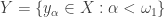
such that $x_\beta \ne x_\gamma$ if $\beta \ne \gamma$ , $x_\alpha \in U_\alpha$ and $x_\alpha \notin \bigcup \limits_{\beta < \alpha} U_\beta$ for each $\alpha < \omega_1$ . At each step $\alpha$ , all the previously chosen open sets cannot cover $Y$ . So we can always choose another point $x_\alpha$ of $Y$ and then choose an open set in $\mathcal{U}$ that contains $x_\alpha$ .

Then $\left\{[\left\{x_\alpha \right\},U_\alpha]: \alpha < \omega_1 \right\}$ is a pairwise disjoint collection of open subsets of $\mathcal{F}[X]$ . Thus if $\mathcal{F}[X]$ has the CCC, then $X$ must be hereditarily Lindelof.

__________________________________

To see bullet point 13, let $Y \subset X$ . Consider open sets $[A,U]$ where $A$ ranges over all finite subsets of $Y$ and $U$ ranges over all open subsets of $X$ with $A \subset U$ . Let $\mathcal{G}$ be a collection of such $[A,U]$ such that $\mathcal{G}$ is pairwise disjoint and $\mathcal{G}$ is maximal (i.e. by adding one more open set, the collection will no longer be pairwise disjoint). We can apply a Zorn lemma argument to obtain such a maximal collection. Let $D$ be the following subset of $Y$ .

$D=\bigcup \left\{A: [A,U] \in \mathcal{G} \text{ for some open } U \right\}$

We claim that the set $D$ is dense in $Y$ . Suppose that there is some open set $W \subset X$ such that $W \cap Y \ne \varnothing$ and $W \cap D=\varnothing$ . Let $y \in W \cap Y$ . Then $[\left\{y \right\},W] \cap [A,U]=\varnothing$ for all $[A,U] \in \mathcal{G}$ . So adding $[\left\{y \right\},W]$ to $\mathcal{G}$ , we still get a pairwise disjoint collection of open sets, contradicting that $\mathcal{G}$ is maximal. So $D$ is dense in $Y$ .

If $\mathcal{F}[X]$ has the CCC, then $\mathcal{G}$ is countable and $D$ is a countable dense subset of $Y$ . Thus if $\mathcal{F}[X]$ has the CCC, the ground space $X$ is hereditarily separable.

__________________________________

A collection $\mathcal{N}$ of subsets of a space $Y$ is said to be a network for the space $Y$ if any non-empty open subset of $Y$ is the union of elements of $\mathcal{N}$ , equivalently, for each $y \in Y$ and for each open $U \subset Y$ with $y \in U$ , there is some $A \in \mathcal{N}$ with $x \in A \subset U$ . Note that a network works like a base but the elements of a network do not have to be open. The concept of network and spaces with countable network are discussed in these previous posts Network Weight of Topological Spaces – I and Network Weight of Topological Spaces – II.

To see bullet point 14, let $\mathcal{N}$ be a network for the ground space $X$ such that $\mathcal{N}$ is also countable. Assume that $\mathcal{N}$ is closed under finite unions (for example, adding all the finite unions if necessary). Let $\left\{[A_\alpha,U_\alpha]: \alpha < \omega_1 \right\}$ be a collection of basic open sets in $\mathcal{F}[X]$ . Then for each $\alpha$ , find $B_\alpha \in \mathcal{N}$ such that $A_\alpha \subset B_\alpha \subset U_\alpha$ . Since $\mathcal{N}$ is countable, there is some $B \in \mathcal{N}$ such that $M=\left\{\alpha< \omega_1: B=B_\alpha \right\}$ is uncountable. It follows that for any finite $E \subset M$ , $\bigcap \limits_{\alpha \in E} [A_\alpha,U_\alpha] \ne \varnothing$ .

Thus if the ground space $X$ has a countable network, then $\mathcal{F}[X]$ has the CCC.

__________________________________

The implications in bullet points 12 and 13 cannot be reversed. Hereditarily Lindelof property and hereditarily separability are not sufficient conditions for $\mathcal{F}[X]$ to have the CCC. See [4] for a study of the CCC property of the Pixley-Roy spaces.

To see bullet point 15, let $S$ be the Sorgenfrey line, i.e. the real line $\mathbb{R}$ with the topology generated by the half closed intervals of the form $[a,b)$ . For each $x \in S$ , let $U_x=[x,x+1)$ . Then $\left\{[ \left\{ x \right\},U_x]: x \in S \right\}$ is a collection of pairwise disjoint open sets in $\mathcal{F}[S]$ .

__________________________________

A Moore space is a space with a development. For the definition, see this previous post.

To see bullet point 16, for each $x \in X$ , let $\left\{B_n(x): n=1,2,3,\cdots \right\}$ be a decreasing local base at $x$ . We define a development for the space $\mathcal{F}[X]$ .

For each finite $F \subset X$ and for each $n$ , let $B_n(F)=\bigcup \limits_{x \in F} B_n(x)$ . Clearly, the sets $B_n(F)$ form a decreasing local base at the finite set $F$ . For each $n$ , let $\mathcal{H}_n$ be the following collection:

$\mathcal{H}_n=\left\{[F,B_n(F)]: F \in \mathcal{F}[X] \right\}$

We claim that $\left\{\mathcal{H}_n: n=1,2,3,\cdots \right\}$ is a development for $\mathcal{F}[X]$ . To this end, let $V$ be open in $\mathcal{F}[X]$ with $F \in V$ . If we make $n$ large enough, we have $[F,B_n(F)] \subset V$ .

For each non-empty proper $G \subset F$ , choose an integer $f(G)$ such that $[F,B_{f(G)}(F)] \subset V$ and $F \not \subset B_{f(G)}(G)$ . Let $m$ be defined by:

$m=\text{max} \left\{f(G): G \ne \varnothing \text{ and } G \subset F \text{ and } G \text{ is proper} \right\}$

We have $F \not \subset B_{m}(G)$ for all non-empty proper $G \subset F$ . Thus $F \notin [G,B_m(G)]$ for all non-empty proper $G \subset F$ . But in $\mathcal{H}_m$ , the only sets that contain $F$ are $[F,B_m(F)]$ and $[G,B_m(G)]$ for all non-empty proper $G \subset F$ . So $[F,B_m(F)]$ is the only set in $\mathcal{H}_m$ that contains $F$ , and clearly $[F,B_m(F)] \subset V$ .

We have shown that for each open $V$ in $\mathcal{F}[X]$ with $F \in V$ , there exists an $m$ such that any open set in $\mathcal{H}_m$ that contains $F$ must be a subset of $V$ . This shows that the $\mathcal{H}_n$ defined above form a development for $\mathcal{F}[X]$ .

____________________________________________________________________

Examples

In the original construction of Pixley and Roy, the example was $\mathcal{F}[\mathbb{R}]$ . Based on the above discussion, $\mathcal{F}[\mathbb{R}]$ is a non-separable CCC Moore space. Because the density (greater than $\omega$ for not separable) and the cellularity ( $=\omega$ for CCC) do not agree, $\mathcal{F}[\mathbb{R}]$ is not metrizable. In fact, it does not even have a dense metrizable subspace. Note that countable subspaces of $\mathcal{F}[\mathbb{R}]$ are metrizable but are not dense. Any uncountable dense subspace of $\mathcal{F}[\mathbb{R}]$ is not separable but has the CCC. Not only $\mathcal{F}[\mathbb{R}]$ is not metrizable, it is not normal. The problem of finding $X \subset \mathbb{R}$ for which $\mathcal{F}[X]$ is normal requires extra set-theoretic axioms beyond ZFC (see [6]). In fact, Pixley-Roy spaces played a large role in the normal Moore space conjecture. Assuming some extra set theory beyond ZFC, there is a subset $M \subset \mathbb{R}$ such that $\mathcal{F}[M]$ is a CCC metacompact normal Moore space that is not metrizable (see Example I in [8]).

On the other hand, Pixley-Roy space of the Sorgenfrey line and the Pixley-Roy space of $\omega_1$ (the first uncountable ordinal with the order topology) are metrizable (see [3]).

The Sorgenfrey line and the first uncountable ordinal are classic examples of topological spaces that demonstrate that topological spaces in general are not as well behaved like metrizable spaces. Yet their Pixley-Roy spaces are nice. The real line and other separable metric spaces are nice spaces that behave well. Yet their Pixley-Roy spaces are very much unlike the ground spaces. This inverse relation between the ground space and the Pixley-Roy space was noted by van Douwen (see [3] and [7]) and is one reason that Pixley-Roy hyperspaces are a good source of counterexamples.

____________________________________________________________________

Reference

Bennett, H. R., Fleissner, W. G., Lutzer, D. J., Metrizability of certain Pixley-Roy spaces, Fund. Math. 110, 51-61, 1980.
Daniels, P, Pixley-Roy Spaces Over Subsets of the Reals, Topology Appl. 29, 93-106, 1988.
Lutzer, D. J., Pixley-Roy topology, Topology Proc. 3, 139-158, 1978.
Hajnal, A., Juahasz, I., When is a Pixley-Roy Hyperspace CCC?, Topology Appl. 13, 33-41, 1982.
Pixley, C., Roy, P., Uncompletable Moore spaces, Proc. Auburn Univ. Conf. Auburn, AL, 1969.
Przymusinski, T., Normality and paracompactness of Pixley-Roy hyperspaces, Fund. Math. 113, 291-297, 1981.
van Douwen, E. K., The Pixley-Roy topology on spaces of subsets, Set-theoretic Topology, Academic Press, New York, 111-134, 1977.
Tall, F. D., Normality versus Collectionwise Normality, Handbook of Set-Theoretic Topology (K. Kunen and J. E. Vaughan, eds), Elsevier Science Publishers B. V., Amsterdam, 685-732, 1984.
Tanaka, H, Normality and hereditary countable paracompactness of Pixley-Roy hyperspaces, Fund. Math. 126, 201-208, 1986.

____________________________________________________________________

$\copyright \ 2014 \text{ by Dan Ma}$

Sorgenfrey Line is not a Moore Space

Posted on September 18, 2012 by Dan Ma

We found an incorrect statement about the Sorgenfrey line in an entry in Wikipedia about Moore space (link). This statement opens up a discussion on the question of whether the Sorgenfrey line is a Moore space as well as a discussion on Moore space. The following is the incorrect statement found in Wikipedia by the author.

5. Neither the Sorgenfrey line nor the Sorgenfrey plane are Moore spaces because they are normal and not second countable

The Sorgenfrey line is the space whose underlying set is the real line $S=\mathbb{R}$ where the topology is generated by a base consisting the half open intervals of the form $[a,b)$ . The Sorgenfrey plane is the square $S \times S$ .

Even though the Sorgenfrey line is normal, the Sorgenfrey plane is not normal. In fact, the Sorgenfrey line is the classic example of a normal space whose square is not normal. Both the Sorgenfrey line and the Sorgenfrey plane are not Moore space but not for the reason given. The statement seems to suggest that any normal Moore space is second countable. But this flies in the face of all the profound mathematics surrounding the normal Moore space conjecture, which is also discussed in the Wikipedia entry.

The statement indicated above is only a lead-in to a discussion of Moore space. We are certain that it will be corrected. We always appreciate readers who kindly alert us to errors found in this blog.

______________________________________________________________________________

Moore Spaces

Let $X$ be a regular space. A development for $X$ is a sequence $\mathcal{G}_1,\mathcal{G}_2,\mathcal{G}_3,\cdots$ of open covers of $X$ such that for each $x \in X$ , and for each open subset $U$ of $X$ with $x \in U$ , there exists one cover $\mathcal{G}_n$ satisfying the condition that for any open set $V \in \mathcal{G}_n$ , $x \in V \Rightarrow V \subset U$ . When $X$ has a development, $X$ is said to be a Moore space (also called developable space). A Note On The Sorgenfrey Line is an introductory note on the Sorgenfrey line.

Moore spaces can be viewed as a generalization of metrizable spaces. Moore spaces are first countable (having a countable base at each point). For a development $\mathcal{G}_1,\mathcal{G}_2,\mathcal{G}_3,\cdots$ , the open sets in $\mathcal{G}_n$ are considered “smaller” as the index $n$ increases. In fact, this is how a development is defined for a metric space, where $\mathcal{G}_n$ consists of all open balls with diameters less than $\frac{1}{n}$ . Thus metric spaces are developable. There are plenty of non-metrizable Moore space. One example is the Niemytzki’s Tangent Disc space.

In a Moore space, every closed set is a $G_\delta$ -set. Thus if a Moore space is normal, it is perfectly normal. Any Moore space has a $G_\delta$ -diagonal (the diagonal $\Delta=\left\{(x,x): x \in X \right\}$ is a $G_\delta$ -set in $X \times X$ ). It is a well known theorem that every compact space with a $G_\delta$ -diagonal is metrizable. Thus any compact Moore space is metrizable.

The last statement can be shown more directly. Suppose that $X$ is compact and has a development $\mathcal{G}_1,\mathcal{G}_2,\mathcal{G}_3,\cdots$ . Then each $\mathcal{G}_n$ has a finite subcover $\mathcal{H}_n$ . Then $\bigcup_{n=1}^\infty \mathcal{H}_n$ is a countable base for $X$ . Thus any compact Moore space is second countable and hence metrizable.

What about paracompact Moore space? Suppose that $X$ is paracompact and has a development $\mathcal{G}_1,\mathcal{G}_2,\mathcal{G}_3,\cdots$ . Then each $\mathcal{G}_n$ has a locally finite open refinement $\mathcal{H}_n$ . Then $\bigcup_{n=1}^\infty \mathcal{H}_n$ is a $\sigma$ -locally finite base for $X$ . The Smirnov-Nagata metrization theorem states that a space is metrizable if and only if it has a $\sigma$ -locally finite base (see Theorem 23.9 on page 170 of [2]). Thus any paracompact Moore space has a $\sigma$ -locally finite base and is thus metrizable (after using the big gun of the Smirnov-Nagata metrization theorem).

______________________________________________________________________________

Sorgenfrey Line

The Sorgenfrey line is regular and Lindelof. Hence it is paracompact. Since the Sorgenfrey line is not metrizable, by the above discussion it cannot be a Moore space. The Sorgenfrey plane is also not a Moore space. Note that being a Moore space is a hereditary property. So if the Sorgenfrey plane is a Moore space, then every subspace of the Sorgenfrey plane (including the Sorgenfrey line) is a Moore space.

The following theorem is another way to show that the Sorgenfrey line is not a Moore space.

Bing’s Metrization Theorem

Every paracompact space is collectionwise normal (see Theorem 5.1.18, p.305 of [1]). Thus the Sorgenfrey line is collectionwise normal and hence cannot be a Moore space. A space $X$ is said to be collectionwise normal if $X$ is a $T_1$ -space and for every discrete collection $\left\{W_\alpha: \alpha \in A \right\}$ of closed sets in $X$ , there exists a discrete collection $\left\{V_\alpha: \alpha \in A \right\}$ of open subsets of $X$ such that $W_\alpha \subset V_\alpha$ . For a proof of Bing’s metrization theorem, see page 329 of [1].

______________________________________________________________________________

Remark

The normal Moore space conjecture is the statement that every normal Moore space is metrizable. This conjecture had been one of the key motivating questions for many set theorists and topologists during a large part of the twentieth century. The bottom line is that this statement cannot not be decided just on the basis of the set of generally accepted axioms called Zermelo–Fraenkel set theory with the axiom of choice, commonly abbreviated ZFC. But Bing’s metrization theorem states that if we strengthen normality to collectionwise normality, we have a definite answer.

______________________________________________________________________________

Reference

Engelking, R., General Topology, Revised and Completed edition, Heldermann Verlag, Berlin, 1989.
Willard, S., General Topology, Addison-Wesley Publishing Company, 1970.

______________________________________________________________________________

$\copyright \ \ 2012$

Completely Regular Spaces and Function Spaces

Posted on August 26, 2012 by Dan Ma

This is a continuation of a discussion on completely regular spaces (continuing from this previous post). These spaces are an integral part of many discussions involving topological spaces and/or properties. Some notions are contingent on the existence of certain real-valued continuous functions. Discussion of such notions can be greatly facilitated by working in the class of completely regular spaces. One example given in a previous post is on a discussion of pseudocompact spaces. Another example for requiring complete regularity is when working with function spaces. When the object being studied is the space of real-valued continuous functions defined on a topological space $X$ , it is desirable to have enough continuous functions in the function space being studied. In this post, we illustrate this point by giving the proofs of two simple results in $C_p(X)$ , the space of real-valued continuous functions endowed with the pointwise convergence topology.

Basic references are [2] and [4]. Refer to [3] for a discussion of where complete regularity is placed among the separation axioms. An in-depth treatment for $C_p$ theory is [1].
________________________________________________________________________

Completely Regular Spaces

A space $X$ is said to be completely regular if $X$ is a $T_0$ space and for each $x \in X$ and for each closed subset $A$ of $X$ with $x \notin A$ , there is a continuous function $f:X \rightarrow [0,1]$ such that $f(A) \subset \left\{0 \right\}$ and $f(x)=1$ . Note that the $T_0$ axiom and the existence of the continuous function imply the $T_1$ axiom, which is equivalent to the property that single points are closed sets. Completely regular spaces are also called Tychonoff spaces.

________________________________________________________________________

Function Spaces

Let $X$ be a space. Let $C(X)$ be the set of all real-valued continuous functions defined on the space $X$ . The set $C(X)$ is naturally a subspace of the product space $\prod \limits_{x \in X} Y_x$ where each $Y_x = \mathbb{R}$ . We can also write $\prod \limits_{x \in X} Y_x = \mathbb{R}^X$ . Thus $C(X)$ can be endowed with the subspace topology inherited from the product space $\mathbb{R}^X$ . When this is the case, the resulting function space is denoted by $C_p(X)$ .

Now we need a good handle on the open sets in the function space $C_p(X)$ . A basic open set in the product space $\mathbb{R}^X$ is of the form $\prod \limits_{x \in X} U_x$ where each $U_x$ is open in $\mathbb{R}$ and $U_x = \mathbb{R}$ for all but finitely many $x \in X$ (equivalently $U_x \ne \mathbb{R}$ for only finitely many $x \in X$ ). Thus a basic open set in $C_p(X)$ is of the form:

$(1) \ \ \ \ \ \ \ \ C(X) \cap \prod \limits_{x \in X} U_x$

where each $U_x$ is open in $\mathbb{R}$ and $U_x = \mathbb{R}$ for all but finitely many $x \in X$ . In addition, when $U_x \ne \mathbb{R}$ , we can take $U_x$ to be an open interval of the form $(a,b)$ . To make the basic open sets of $C_p(X)$ more explicit, $(1)$ is translated as follows:

$(2) \ \ \ \ \ \ \ \ \bigcap \limits_{x \in F} [x, O_x]$

where $F \subset X$ is a finite set, for each $x \in F$ , $O_x$ is an open interval of $\mathbb{R}$ , and $[x,O_x]$ is the set of all $f \in C(X)$ such that $f(x) \in O_x$ . In proving results about $C_p(X)$ , we can use basic open sets that are described in $(2)$ .

________________________________________________________________________

Completely Regular Spaces and Function Spaces

We now give two simple results in $C_p(X)$ that are good illustrations that complete regularity is the ideal setting for the domain space of $C_p$ function spaces. In Theorem 1, complete regularity is used to generate a non-separable subspace of the function space given a non-Lindelof subspace of the domain space. In Theorem 2, complete regularity is used to generate a non-Lindelof subspace of the function space given a non-separable subspace of the domain space.

Theorem 1
Let $X$ be a completely regular space. Then if $C_p(X)$ is hereditarily separable, then $X$ is hereditarily Lindelof.

Proof
We show that if $X$ has a subspace that is not Lindelof, then there is a subspace of $C_p(X)$ that is not separable. We use complete regularity to generate the continuous functions that form a non-separable subspace.

Let $Y \subset X$ be a non-Lindelof subspace. There exists an open cover $\mathcal{U}$ of $Y$ such that $\mathcal{U}$ has no countable subcover. Open sets in $\mathcal{U}$ are open sets in $Y$ . We wish to expand these to open sets in $X$ . Let $\mathcal{U}^*$ be the collection of open subsets $U$ of $X$ such that $U \cap Y \in \mathcal{U}$ . It is clear that no countable subcollection of $\mathcal{U}^*$ can cover $Y$ .

For each $y \in Y$ , choose $U(y) \in \mathcal{U}^*$ such that $y \in U(y)$ . Here’s where we use complete regularity. For each $y \in Y$ , there is a continuous function $f_y:X \rightarrow [0,1]$ such that $f_y(X-U(y)) \subset \left\{0 \right\}$ and $f_y(y) =1$ . Let $T=\left\{f_y:y \in Y \right\}$ , which is a subspace of $C_p(X)$ .

We claim that $T$ is not separable. To see this, let $A=\left\{g_1,g_2,g_3,\cdots \right\}$ be a countable subset of $T$ such that for each $i$ , $g_i$ is obtained from the point $y(i) \in Y$ and the open set $U_i=U(y(i))$ , i.e., $g_i=f_{y(i)}$ . Note that $\left\{U_1,U_2,U_3,\cdots \right\}$ cannot be a cover of $Y$ . Let $a \in Y$ be a point that is not in all $U_i$ .

Consider the function $f_a$ chosen above using complete regularity. Note that $f_a(a)=1$ and $f_a(X-U(a)) \subset \left\{0 \right\}$ . On the other hand, $g_i(a)=f_{y(i)}(a)=0$ for all $i$ since $a \notin U_i$ for all $i$ . This means that $f_a$ is not in the closure of $A$ . For example, $[a,(0.9,1.1)]$ is a basic open set containing $f_a$ such that $g_i \notin [a,(0.9,1.1)]$ for all $i$ . Thus no countable subset of $T$ can be dense in $T$ , completing the proof. $\blacksquare$

Theorem 2
Let $X$ be a completely regular space. Then if $C_p(X)$ is hereditarily Lindelof, then $X$ is hereditarily separable.

Proof
Let $Y$ be a non-separable subspace of $X$ . For each countable $A \subset Y$ , there must be some point $y(A) \in Y$ such that $y(A)$ is not a member of the closure of $A$ (relative to $Y$ ). For each countable $A \subset Y$ , let $\overline{A}$ be the closure of $A$ in the entire space $X$ . Clearly $y(A) \notin \overline{A}$ .

Now apply the complete regularity of the space $X$ . For each countable $A \subset Y$ , let $f_A: X \rightarrow [0,1]$ be continuous such that $f_A(\overline{A}) \subset \left\{0 \right\}$ and $f_A(y(A))=1$ . Let $W$ be the set of all $f_A$ where $A \subset Y$ is countable.

We now show that $W$ is a non-Lindelof subspace of $C_p(X)$ . For each $f_A \in W$ , let $U_A=[y(A),(0.9, 1.1)] \cap W$ , which is open in $C_p(X)$ and contains $f_A$ . Let $\mathcal{U}$ be the collection of all such open sets $U_A$ .

Then $\mathcal{U}$ is an open cover of $W$ that has no countable subcover. To see this, suppose we have $\left\{U_1,U_2,U_3,\cdots \right\}$ such that for each $i$ , $U_i=U_{A(i)}$ where $A(i) \subset Y$ is countable. Then let $B$ be the set of all $A(i)$ and all points $y(A(i))$ . Note that the set $B$ is still a countable subset of $Y$ . Consider the point $y(B)$ and the continuous function $f_B$ , which is a member of $W$ . We have $f_B(y(B))=1$ and $f_B(t)=0$ for all $t \in \overline{B}$ . Note that each $y(A(i)) \in B$ and thus $f_B(y(A(i))=0$ for all $i$ . This shows that $f_B \notin U_i=U_{A(i)}$ for all $i$ . Then $\mathcal{U}$ is an open cover of $W$ that has no countable subcover, leading to the conclusion that $W$ is a non-Lindelof subspace of $C_p(X)$ . $\blacksquare$

________________________________________________________________________

Remark

The above proofs of Theorem 1 and Theorem 2 are only meant as demonstration of the role played by complete regularity in working with function spaces. They are much weaker versions of a deeper result. These two results can serve to motivate a deeper result that explores the relationship between the hereditary separability (respectively hereditary Lindelof property) of the domain space and the hereditary Lindelof property (respectively the hereditary separability) of the function space. The following theorem is the countable version of a theorem found in [5].

Theorem 3
Let $X$ be a completely regular space. The following conditions are equivalent.

$C_p(X)$ is hereditarily separable (respectively hereditarily Lindelof).
$X^\omega$ is hereditarily Lindelof (respectively hereditarily separable).
For each positive integer $n$ , $X^n$ is hereditarily Lindelof (respectively hereditarily separable).

________________________________________________________________________

Reference

Arhangel’skii, A., Topological Function Spaces, Kluwer Academic Publishers, Boston, 1992.
Engelking, R., General Topology, Revised and Completed edition, Heldermann Verlag, Berlin, 1989.
Steen, L. A., Seebach, J. A., Counterexamples in Topology, Dover Publications, Inc., New York, 1995.
Willard, S., General Topology, Addison-Wesley Publishing Company, 1970.
Zenor, P., Hereditarily m-separability and the hereditarily m-lindelof property in product spaces and function spaces, Fund. Math. 106, 175-180, 1980.

Thinking about the Space of Irrationals Topologically

Posted on May 13, 2012 by Dan Ma

Let $\mathbb{R}$ denote the real number line and $\mathbb{P}$ denote the set of all irrational numbers. The irrational numbers and the set $\mathbb{P}$ occupy an important place in mathematics. The set $\mathbb{P}$ with the Euclidean topology inherited from the full real line is a topological space in its own right. Thus the space $\mathbb{P}$ has some of the same properties inherited from the Euclidean real line, e.g., just to name a few, it is hereditarily separable, hereditarily Lindelof, paracompact and metrizable. The space of the irrational numbers $\mathbb{P}$ has many properties apart from the full real line (e.g. $\mathbb{P}$ is totally disconnected). In this post, we look at a topological description of the space $\mathbb{P}$ .

Let $\omega$ be the set of all nonnegative integers. Then the space $\mathbb{P}$ of irrational numbers is topologically equivalent (i.e. homeomorphic to) the product space $\prod \limits_{i=0}^\infty X_i$ where each $X_i=\omega$ has the discrete topology. We will also denote the product space $\prod \limits_{i=0}^\infty X_i$ by $\omega^\omega$ . We have the following theorem.

Theorem
The space $\mathbb{P}$ of irrational numbers is homeomorphic to the product space $\omega^\omega$ .

Because of this theorem, we can look at irrational numbers as sequences of nonnegative integers. Specifically each irrational number can be identified by a unique sequence of nonnegative integers. We can think of each such unique sequence as an address to locate an irrational number. In the remainder of the post, we describe at a high level how to define the unique addresses, which will also give us a homeomorphic map between the space $\mathbb{P}$ and the product space $\omega^\omega$ .

___________________________________________________________________________

Step 0
Put the rational numbers in a sequence $r_0,r_1,r_2,r_3,\cdots$ such that $r_0=0$ . We divide the real line into countably many non-overlapping intervals. Specifically, let $A_0=[0,1]$ , $A_1=[-1,0]$ , $A_2=[1,2]$ , etc (see the following figure).

To facilitate the remaining construction, we denote the left endpoint of the interval $A_i$ by $L_i$ and denote the right endpoint by $R_i$ .

Step 1
In each of the interval $A_i$ , we further divide it into non-overlapping intervals. The left endpoint and the right endpoint of the interval $A_i$ are $L_i$ and $R_i$ , respectively. We choose a sequence $x_{i,0}, x_{i,1}, x_{i,2},\cdots$ of rational numbers converging to the right endpoint $R_i$ . Then let $A_{i,0}=[L_i,x_{i,0}]$ , $A_{i,1}=[x_{i,0},x_{i,1}]$ , $A_{i,2}=[x_{i,1},x_{i,2}]$ , etc (see the following figure).

Two important points to consider in Step $1$ . One is that we make sure the rational number $r_1$ is chosen as an endpoint of some interval in Step 1. The second is that the length of each $A_{i,j}$ is less than $\displaystyle \frac{1}{2^1}$ .

Step 2
In each of the interval $A_{i,j}$ , we further divide it into non-overlapping intervals. The left endpoint and the right endpoint of the interval $A_{i,j}$ are $L_{i,j}$ and $R_{i,j}$ , respectively. We choose a sequence $x_{i,j,0}, x_{i,j,1}, x_{i,j,2},\cdots$ of rational numbers converging to the left endpoint $L_{i,j}$ . Then let $A_{i,j,0}=[x_{i,j,0},R_{i,j}]$ , $A_{i,j,1}=[x_{i,j,1},x_{i,j,0}]$ , $A_{i,j,2}=[x_{i,j,2},x_{i,j,1}]$ , etc (see the following figure).

As in the previous step, two important points to consider in Step $2$ . One is that we make sure the rational number $r_2$ is chosen as an endpoint of some interval in Step 2. The second is that the length of each $A_{i,j,k}$ is less than $\displaystyle \frac{1}{2^2}$ .

___________________________________________________________________________
Remark

In the process described above, the endpoints of the intervals $A_{f(0),\cdots,f(n)}$ are rational numbers and we make sure that all the rational numbers are used as endpoints. We also make sure that the intervals from the successive steps are nested closed intervals with lengths $\rightarrow 0$ . The consequence of this point is that the nested decreasing closed intervals will collapse to one single point (since the real line is a complete metric space) and this single point must be an irrational number (since all the rational numbers are used up as endpoints of the nested closed intervals).

In Step $i$ where $i$ is an odd integer, we make the endpoints of the new intervals converge to the right. In Step $i$ where $i>1$ is an even integer, we make the endpoints of the new intervals converge to the left. This manipulation is to ensure that the nested closed intervals will never share the same endpoint from one step all the way to the end of the process.

Thus if we have $f \in \omega^\omega$ , then $\bigcap \limits_{n=0}^\infty A_{f(0),\cdots,f(n)} \ne \varnothing$ and in fact has only one point that is an irrational number.

On the other hand, for each point $x \in \mathbb{P}$ , we can locate inductively a sequence of intervals, $A_{f(0)}, A_{f(0),f(1)}, A_{f(0),f(1),f(2)}, \cdots$ , containing the point $x$ . This sequence of nested closed intervals must collapse to a single point and the single point must be the irrational number $x$ .

The process described above gives us a one-to-one mapping from $\mathbb{P}$ onto the product space $\omega^\omega$ . This mapping is also continuous in both directions, making it a homeomorphism. the nested intervals defined above form a base for the Euclidean topology on $\mathbb{P}$ . These basic open sets have a natural correspondance with basic open sets in the product space $\omega^\omega$ .

For example, for $f \in \omega^\omega$ , $\left\{ A_{f(0),\cdots,f(n)} \cap \mathbb{P}: n \in \omega \right\}$ is a local base at the point $x \in \bigcap \limits_{n=0}^\infty A_{f(0),\cdots,f(n)}$ . One the other hand, each $A_{f(0),\cdots,f(n)} \cap \mathbb{P}$ has a natural counterpart in a basic open set in the product space, namely the following set:

$\displaystyle . \ \ \ \ \left\{g \in \omega^\omega: g \restriction n = f \restriction n \right\}$

___________________________________________________________________________

The above process establishes that the countable product of the integers, $\omega^\omega$ , is equivalent topologically to the Euclidean space $\mathbb{P}$ .

When is a Lindelof Space Normal?

Posted on May 3, 2012 by Dan Ma

When is a Lindelof space normal? This question may seem strange since it is a well known basic result that Lindelof spaces are normal (see Theorem 3.8.2 in [1] and Theorem 16.8 in [6]). The proofs in both of these theorems require that the Lindelof space is also a regular space. We present an example showing that the requirement of regularity cannot be removed. The example defined below is a space that is Hausdorff, hereditarily Lindelof, not separable, not regular and not normal.

The example defined below makes it clear that we need to be careful in making the leap from the Lindelof property to normality of a space. We need to make sure that the space in question is also a regular space. The Lindelof property is a powerful property; it also implies paracompactness. But for this to happen, some separation axiom is required (it needs to be a regular space).

Another motivation for looking at examples such as the one defined here is that they are background information to the theory of S-spaces and L-spaces (see the remark given at the end of the post).

______________________________________________________________________________

The example is the Example 14.7 in [2]. The underlying set is the real number line $\mathbb{R}$ . Let $\tau$ be the usual topology on $\mathbb{R}$ . Let $X=\mathbb{R}$ . We use the following collection of sets as a base for a new topology on $X$ :

$\displaystyle \mathbb{B}=\left\{O-C: O \in \tau, C \subset \mathbb{R}, \lvert C \vert \le \omega \right\}$

The collection $\mathbb{B}$ needs to satisfy two conditions for being a base for a topology. One is that it covers the underlying set. The second is that whenever $B_1, B_2 \in \mathbb{B}$ with $x \in B_1 \cap B_2$ , there is some $B_3 \in \mathbb{B}$ such that $x \in B_3 \subset B_1 \cap B_2$ . Note that $\tau \subset \mathbb{B}$ . This implies that $\mathbb{B}$ is a cover of $X$ . It is also clear that the second condition is satisfied.

Let $\tau^{*}$ be the topology generated by the base $\mathbb{B}$ . Another consequence of $\tau \subset \mathbb{B}$ is that the new topology on $X$ is finer than the usual topology, i.e., $\tau \subset \tau^{*}$ . It is then clear that $(X, \tau^{*})$ is a Hausdorff space.

We denote the real line with the new topology $\tau^{*}$ by $X$ rather than $(X, \tau^{*})$ since the new topology $\tau^{*}$ is the primary focus.

In $X$ , the complement of every countable set is open. So no countable set can be dense in $X$ , making it not separable. Equivalently, every countable subset of $X$ is closed.

To see that $X$ is not regular, we first make the following observation.

Observation
Let $W \subset \mathbb{R}$ be a Euclidean open set. Let $A \subset \mathbb{R}$ be a countable set that is dense in $W$ (dense with respect to the Euclidean topology). Then for each $x \in A \cap W$ , $x \in \overline{W-A}$ (with respect to the topology $\tau^*$ ).

To see that this observation is correct, let $x \in A \cap W$ and let $V-B$ be an open set containing $x$ , where $V$ is a Euclidean open set and $B$ is a countable set. We can assume that $V \subset W$ . Let $A_0=A-\left\{x \right\}$ . Note that $x \in V-(A_0 \cup B) \subset V-B$ and that $V-(A_0 \cup B) \subset W-A_0$ . Furthermore, for any $y \in V-(A_0 \cup B)$ with $y \ne x$ , $y \in W-A$ . Thus any open set containing $x$ contains many points of $W-A$ . Hence, we have $x \in \overline{W-A}$ .

To see that $X$ is not regular, we show that there is a closed set $C \subset X$ such that for any open set $O \subset X-C$ , $\overline{O} \cap C \ne \varnothing$ .

Let $C=\mathbb{Q}$ (the set of all rational numbers). Let $O$ be open in $X$ such that $O \subset X-C$ . We assume that $O=W-A$ where $W$ is open in the Euclidean topology and $A$ is countable. Note that $O=W-A$ consisting of entirely of irrational numbers. Then $\mathbb{Q} \cap W \subset A$ . Thus $A$ is dense in $W$ (with respect to the Euclidean topology). By the above observation, any point of $A$ is a member of $\overline{W-A}$ (with respect to the topology $\tau^*$ ). In particular, for each $x \in C=\mathbb{Q}$ , $x \in \overline{W-A}$ . Thus $X$ is not regular.

Any space that is not regular is also not normal. Thus $X$ is not normal. But we can also see this directly. Let $H=\mathbb{Q}$ and $K=\left\{x \right\}$ where $x$ is any irrational number. Then $H$ and $K$ are two disjoint closed sets that cannot be separated by disjoint open sets in $X$ .

The space $X$ is Lindelof and also hereditarily Lindelof (both properties are piggy backed on the same properties of the Euclidean real line). To see that $X$ is Lindelof, suppose that a collection of open sets $O_a-A_a \in \mathbb{B}$ is a cover of $X$ . The Euclidean open sets $O_a$ also form a cover of $X=\mathbb{R}$ . Then pick countably many $O_a$ that also cover the real line (using the Lindelof property of the Euclidean real line). Then these countably many $O_a-A_a$ will cover $X$ except for countably many points. A countable subcover will result once we use open sets in the original cover to cover these countably many points. Using the same proof, it can be shown that every subspace of $X$ is also Lindelof.

______________________________________________________________________________

Remark

An S-space is any regular topological space that is hereditarily separable but not Lindelof. An L-space is any regular topological space that is hereditarily Lindelof but not separable. Elementary examples of hereditarily separable space that is not Lindelof and hereditarily Lindelof space that is not separable are quite easy to define (but they are not regular). The example we define above is an example of non-regular hereditarily Lindelof space that is not separable. Thus S-space and L-space are typically defined with the requirement of regularity.

It was shown in the early 1980’s that the existence of S-space is independent of the usual axioms of ZFC. This means that to prove the existence of an S-space or to prove the non-existence of S-space, one needs to assume axioms beyond those of ZFC. The L-space problem (whether an L-space can exist without assuming additional set-theoretic assumptions beyond those of ZFC) was not resolved until quite recently. For quite a long time, it was believed the L-space problem would have a similar solution (that its existence would be independent of ZFC). In 2005, Justin Tatch-Moore solved the L-space problem by constructing an L-space without assuming additional axioms.

For back ground information about S-space and L-space, see [3] and [4]. For Justin Moore’s proof, see [5].

______________________________________________________________________________

Reference

Engelking, R., General Topology, Revised and Completed edition, 1989, Heldermann Verlag, Berlin.
Hodel, R.,Cardinal Functions I, Handbook of Set-Theoretic Topology, (K. Kunen and J. E. Vaughan, eds), 1984, Elsevier Science Publishers B. V., Amsterdam, 1-61.
Mastros, S.,S and L Spaces, Master’s Thesis, 2009, University of Pittsburgh. Link
Roitman, J.,Basic S and L, Handbook of Set-Theoretic Topology, (K. Kunen and J. E. Vaughan, eds), 1984, Elsevier Science Publishers B. V., Amsterdam, 295-326.
Tatch-Moore, J.,A solution to the L space problem, Journal of the American Mathematical Society, 19 (2006), 3, 717—736. Link
Willard, S., General Topology, 1970, Addison-Wesley Publishing Company.

An observation about hereditarily separable function spaces

Posted on April 9, 2011 by Dan Ma

For any completely regular space $X$ , by $C_p(X)$ we mean the space of all real-valued continuous functions on $X$ endowed with the pointwise convergent topology. It is known that $C_p(X)$ is hereditarily separable if and only if $X^n$ is hereditarily Lindelof for all positive integer $n$ if and only if $X^\omega$ is hereditarily Lindelof where $\omega$ is the first infinite ordinal (a result that follows from a theorem of Zenor in [4]). This result points to a duality between hereditary separability of the function space $C_p(X)$ and the hereditary Lindelof property of the domain space $X$ and is restated below.

Theorem
Let $X$ be a completely regular space. Then the following conditions are equivalent:

$C_p(X)$ is hereditarily separable.
$X^n$ is hereditarily Lindelof for all positive integer $n$ .
$X^\omega$ is hereditarily Lindelof.

As an introduction to this theorem, we present the proof to one direction of this theorem for $n=1$ .

Observation
Let $X$ be any completely regular space. We have the following obervation:

If $C_p(X)$ is hereditarily separable, then $X$ is hereditarily Lindelof.

Suppose $X$ is not hereditarily Lindelof. We aim to show that $C_p(X)$ is not hereditarily separable by producing a non-separable subspace $\mathcal{F}$ of $C_p(X)$ .

Let $Y \subset X$ be a subspace that is not Lindelof. Let $\mathcal{U}$ be a collection of open subsets of $X$ such that $\mathcal{U}$ covers $Y$ and no countable subcollection of $\mathcal{U}$ covers $Y$ .

For each $y \in Y$ , choose $U_y \in \mathcal{U}$ such that $y \in U_y$ . By the completely regularity of $X$ , choose a continuous $f_y: X \rightarrow \mathbb{R}$ such that $f_y$ maps $X-U_y$ to $0$ and $f_y(y)=1$ . Let $\mathcal{F}=\left\{f_y:y \in X \right\}$ . It can be shown that $\mathcal{F}$ is a non-separable subspace of $C_p(X)$ . That is, no countable subset of $\mathcal{F}$ can be dense in $\mathcal{F}$ . $\blacksquare$

For any completely regular space $X$ , it is also known (see [2]) that $C_p(X)$ is separable if and only if $X$ has a weaker separable metrizable topology (i.e. $X$ has a weaker topology such that $X$ with this weaker topology is a separable metrizable space). The result in [2] combined with the observation presented here provides a way to obtain sepearable $C_p(X)$ that is not hereditarily separable. Look for any $X$ that is not hereditarily Lindelof but has a weaker separable metrizable topology. One such example is the Michael Line.

The observation we make here is a rather weak result. The double arrow space $Z$ is hereditarily Lindelof. Yet $C_p(Z)$ is not even separable since $Z$ is compact space that is not metrizable. Note that $Z^2$ is not hereditarily Lindelof since it contains a copy of the Sorgenfrey plane (see the previous post on double arrow space).

Reference

Engelking, R., General Topology, Revised and Completed edition, 1989, Heldermann Verlag, Berlin.
Noble, N., The density character of function spaces, Proc. Amer. Math. Soc. 42:1 (1974) 228-233.
Willard, S., General Topology, 1970, Addison-Wesley Publishing Company.
Zenor, P., Hereditarily m-separability and the hereditarily m-lindelof property in product spaces and function spaces, Fund. Math. 106 (1980), 175-180

Spaces With Countable Network

Posted on November 14, 2009 by Dan Ma

The concept of network is a useful tool in working with generalized metric spaces. A network is like a base for a topology, but the members of a network do not have to be open. After a brief discussion on network, the focus here is on the spaces with networks that are countably infinite in size. The following facts are presented:

Any space with a countable network is separable and Lindelof.
The property of having a countable network is hereditary. Thus any space with a countable network is hereditarily separable and hereditarily Lindelof.
The property of having a countable network is preserved by taking countable product.
The Sorgenfrey Line is an example of a hereditarily separable and hereditarily Lindelof space that has no countable network.
For any compact space $X$ , $nw(X)=w(X)$ . In particular, any compact space with a countable network is metrizable.
As a corollary to 5, $w(X) \leq \vert X \vert$ for any compact $X$ .
A space $X$ has a countable network if and only if it is the continuous impage of a separable metric space (hence such a space is sometimes called cosmic).
Any continuous image of a cosmic space is cosmic.
Any continuous image of a compact metric space is a compact metric space.
As a corollary to 2, any space with countable network is perfectly normal.
An example is given to show that the continuous image of a separable metric space needs not be metric (i.e. an example of a cosmic space that is not metrizable).

All spaces in this discussion are at least $T_3$ (Hausdorff and regular). Let $X$ be a space. A collection $\mathcal{N}$ of subsets of $X$ is said to be a network for $X$ if for each $x \in X$ and for each open $U \subset X$ with $x \in U$ , then we have $x \in N \subset U$ for some $N \in \mathcal{N}$ . The network weight of a space $X$ , denoted by $nw(X)$ , is defined as the minimum cardinality of all the possible $\vert \mathcal{N} \vert$ where $\mathcal{N}$ is a network for $X$ . The weight of a space $X$ , denoted by $w(X)$ , is defined as the minimum cardinality of all possible $\vert \mathcal{B} \vert$ where $\mathcal{B}$ is a base for $X$ . Obviously any base is also a network. Thus $nw(X) \leq w(X)$ . For any compact space $X$ , $nw(X)=w(X)$ . On the other hand, the set of singleton sets is a network. Thus $nw(X) \leq \vert X \vert$ .

Our discussion is based on an important observation. Let $\mathcal{T}$ be the topology for the space $X$ . Let $\mathcal{K}=nw(X)$ . We can find a base $\mathcal{B}_0$ that generates a weaker (coarser) topology such that $\lvert \mathcal{B}_0 \lvert=\mathcal{K}$ . We can also find a base $\mathcal{B}_1$ that generates a finer topology such that $\lvert \mathcal{B}_1 \lvert=\mathcal{K}$ . These are restated as lemmas.

Lemma 1. We can define base $\mathcal{B}_0$ that generates a weaker (coarser) topology $\mathcal{S}_0$ on $X$ such that $\lvert \mathcal{B}_0 \lvert=\mathcal{K}$ . Thus $w(X,\mathcal{S}_0) \leq nw(X)$ .

Proof. Let $\mathcal{N}$ be a network for $(X,\mathcal{T})$ such that $\vert \mathcal{N} \vert=nw(X,\mathcal{T})$ . Consider all pairs $N_0,N_1 \in \mathcal{N}$ such that there exist disjoint $O_0,O_1 \in \mathcal{T}$ with $N_0 \subset O_0$ and $N_1 \subset O_1$ . Such pairs exist because we are working in a Hausdorff space. Let $\mathcal{B}_0$ be the collection of all such open sets $O_0,O_1$ and their finite interections. This is a base for a topology and let $\mathcal{S}_0$ be the topology generated by $\mathcal{B}_0$ . Clearly, $\mathcal{S}_0 \subset \mathcal{T}$ and this is a Hausdorff topology. Note that $w(X,\mathcal{S}_0) \leq \vert \mathcal{B}_0 \vert =\vert \mathcal{N} \vert$ .

Lemma 2. We can define base $\mathcal{B}_1$ that generates a finer topology $\mathcal{S}_1$ on $X$ such that $\lvert \mathcal{B}_1 \lvert=\mathcal{K}$ . Thus $w(X,\mathcal{S}_1) \leq nw(X)$ .

Proof. As before, let $\mathcal{N}$ be a network for $(X,\mathcal{T})$ such that $\vert \mathcal{N} \vert=nw(X,\mathcal{T})$ . Since we are working in a regular space, we can assume that the sets in $\mathcal{N}$ are closed. If not, take closures of the elements of $\mathcal{N}$ and we still have a network. Consider $\mathcal{B}_1$ to be the set of all finite intersections of elements in $\mathcal{N}$ . This is a base for a topology on $X$ . Let $\mathcal{S}_1$ be the topology generated by this base. Clearly, $\mathcal{T} \subset \mathcal{S}_1$ . It is also clear that $w(X,\mathcal{S}_1) \leq nw(X)$ . The only thing left to show is that the finer topology is regular. Note that the network $\mathcal{N}$ consists of closed sets in the topology $\mathcal{T}$ . Thus the sets in the base $\mathcal{B}_1$ also consists of closed sets with respect to $\mathcal{T}$ and the sets in $\mathcal{B}_1$ are thus closed in the finer topology. Since $\mathcal{B}_1$ is a base consisting of cloased and open sets, the topology $\mathcal{S}_1$ regular.

Discussion of 1, 2, and 3
Points 1, 2 and 3 are basic facts about countable network and they are easily verified based on definitions. They are called out for the sake of having a record.

Discussion of 4
The Sorgenfrey Line does not have a countable network for the same reason that the Sorgenfrey Plane is not Lindelof. If the Sorgenfrey Line has a countable netowrk, then the Sorgenfrey plane would have a countable network and hence Lindelof.

Discussion of 5
In general, $nw(X) \leq w(X)$ . In a compact Hausdorff space, any weaker Hausdorff topology must conincide with the original topology. So the weaker topology produced in Lemma 1 must coincide with the original topology. In the countable case, any compact space with a countable network has a weaker topology with a countable base. This weaker topology must coincide with the original topology.

Discussion of 6
Note that $nw(X) \leq \lvert X \lvert$ always holds. For compact spaces, we have $w(X)=nw(X) \leq \lvert X \lvert$ .

Discussion of 7
Let $X$ be a space with a countable network. By Lemma 2, $X$ has a finer topology that has a countable base. Let $Y$ denote $X$ with this finer second countable topology. Then the identity map from $Y$ onto $X$ is continuous.

For the other direction, let $f:Y \rightarrow X$ be a continuous function mapping a separable metric space $Y$ onto $X$ . Let $\mathcal{B}$ be a countable base for $Y$ . Then $\lbrace{f(B):B \in \mathcal{B}}\rbrace$ is a network for $X$ .

Discussion of 8
This is easily verified. Let $X$ is the continuous image of a cosmic space $Y$ . Then $Y$ is the continuous image of some separable metric space $Z$ . It follows that $X$ is the continuous image of $Z$ .

Discussion of 9
Let $X$ be compact metrizable and let $Y$ be a continuous image of $X$ . Then $Y$ is compact. By point 7, $Y$ has a countable network. By point 5, $Y$ is metrizable.

Discussion of 10
A space is perfectly normal if it is normal and that every closed subset is a $G_\delta-$ set. Let $X$ be a space with a countable network. The normality of $X$ comes from the fact that it is regular and Lindelof. Note that $X$ is also hereditarily Lindelof. In a hereditarily Lindelof and regular space, every open subspace is an $F_\sigma-$ set (thus every closed set is a $G_\delta-$ set.

Discussion of 11 (Example of cosmic but not separable metrizable space)
This is the “Butterfly” space or “Bow-tie” space due to L. F. McAuley. I found this example in [Michael]. Let $Y=T \cup S$ where
$T=\lbrace{(x,y) \in \mathbb{R}^2:y>0}\rbrace$ and
$S=\lbrace{(x,y) \in \mathbb{R}^2:y=0}\rbrace$ .

Points in $T$ have the usual plane open neighborhoods. A basic open set at $p \in S$ is of the form $B_c(p)$ where $B_c(p)$ consists of $p$ and all points $q \in Y$ having distance $<c$ from $p$ and lying underneath either one of the two straight lines in $Y$ which emanate from $p$ and have slopes $+c$ and $-c$ , respectively.

It is clear that $Y$ is a Hausdorff and regular space. The relative “Bow-tie” topologies on $T$ and $S$ coincide with the usual topology on $T$ and $S$ , respectively. Thus the union of the usual countable bases on $T$ and $S$ would be a countable network for $Y$ . On the other hand, $Y$ is separable but cannot have a countable base (hence not metrizable).

Reference
[Michael]
Michael, E., $\aleph_0-$ spaces, J. Math. Mech. 15, 983-1002.

Product of Separable Spaces

Posted on November 6, 2009 by Dan Ma

In [Ross & Stone], it was shown that the product of $\leq$ continuum many separable spaces is separable while the product of more than continuum many separable spaces is not separable. My goal here is to write down a proof here as a record for future reference. While the product of continuum many separable factors is separable, it can never be hereditarily separable. Any product space with uncountably many factors, each of which has at least two points, has a subspace that is not separable. The non-separable subspace shown here is the $\Sigma-$ product. The $\Sigma-$ product of $\leq$ continuum (but uncountably) many separable spaces is an example of a space with the countable chain condition (ccc) that is not separable.

A. The Product of Continuum Many Separable Spaces
Suppose that $X_a$ is a separable space for each $a \in \mathbb{R}$ . Then the product space $Y=\Pi_{a \in \mathbb{R}} X_a$ is separable.

Proof. The proof uses the fact that the real line $\mathbb{R}$ has a countable base. Let $\omega$ be the set of all natural numbers. For each $a \in \mathbb{R}$ , let $\lbrace{x_{a,0},x_{a,1},x_{a,2},...}\rbrace$ be a countable dense subset of $X_a$ . Let $\mathcal{B}$ be the collection of all open intervals in $\mathbb{R}$ with rational endpoints.

Let $F$ be a pairwise disjoint finite collection of $\mathcal{B}$ . Fix a function $f:F \rightarrow \omega$ . For this $(F,f)$ combination, we define a point $h \in Y$ . For each open interval $B \in F$ , $h(a)=x_{a,f(B)}$ for all points $a \in B$ . For all other $a \in \mathbb{R}$ , define $h(a)=x_{a,0}$ . Since there are only countably many $(F,f)$ combinations, this algorithm defines a countable subspace $D$ of the product space $Y$ . It follows that $D$ is dense in $Y$ .

Comment
If there are $\mathcal{K}$ many factors where $\mathcal{K} \leq$ continuum, just use a subspace of the real line with cardinality $\mathcal{K}$ as an index set. Then choose a countable base of the index set and apply the same proof.

B. The Product of Greater Than Continuum Many Separable Spaces
Suppose that for each $a \in \mathbb{S}$ , $X_a$ is a separable space with at least two points. If the product space $Y=\Pi_{a \in S} X_a$ is separable, then $\vert S \vert \leq \vert \mathbb{R} \vert$ . Thus if the cardinality of the index set $S$ is greater than continuum, then the product space can never be separable.

Proof. For each $a \in S$ , choose two disjoint nonempty open sets $U_{a,0},U_{a,1}$ in $X_a$ . This is possible since $X_a$ has at least two points and is a Hausdorff space. Let $D$ be a countable dense subset of the product space $Y$ . For each $a \in S$ , define $D_a=\lbrace{h \in Y:h(a) \in U_{a,0}}\rbrace \cap D$ . Each $D_a$ is nonempty because it is the intersection of an open set with a dense set. For $a \neq b$ , $D_a \neq D_b$ . So here is a one-to-one mapping of $S$ into the power set of the countable set $D$ . Thus $\vert S \vert \leq \vert \mathbb{R} \vert$ .

C. The Product Space With Uncountably Many Factors Is Not Hereditarily Separable

Proof. Suppose that we have a product space $Y=\Pi_{a \in S} X_a$ where $S$ is uncountable and each factor has at least two points. Given a point $p \in Y$ , the $\Sigma-$ product is the following subspace of the product space $Y$ :

$\Sigma_{a \in S} X_a=\lbrace{h \in Y:h(a) \neq p(a)}$ for only countably many $a \in S\rbrace$ .

Let $\lbrace{h_0,h_1,h_3,...}\rbrace$ be a countable subset of $\Sigma_{a \in S} X_a$ . Since each point $h_i$ disagrees with $p$ at only countably many points, choose one $b \in S$ such that each $h_i(b)=p(b)$ . Then consider the open set $V=\lbrace{h \in \Sigma_{a \in S} X_a:h(b) \in W}\rbrace$ where $W$ is open in $X_b$ such that and $p(b) \notin W$ . None of the $h_i$ belongs to $V$ .

Comment
The $\Sigma-$ product $\Sigma_{a \in S} X_a$ of $\leq$ continuum (but uncountably) many separable spaces is an example of “ccc and not separable”.

Reference
[Ross & Stone] Ross, K. A., Stone, A. H. [1964] Product of Separable Spaces, The American Mathematical Monthly, Vol. 71, pp. 398-403.

Dan Ma's Topology Blog

Expository Articles In General Topology

Tag Archives: Hereditarily separable

A little corner in the world of set-theoretic topology

Cp(X) where X is a separable metric space

Pixley-Roy hyperspaces

Sorgenfrey Line is not a Moore Space

Completely Regular Spaces and Function Spaces

Thinking about the Space of Irrationals Topologically

When is a Lindelof Space Normal?

An observation about hereditarily separable function spaces

Spaces With Countable Network

Product of Separable Spaces