Drawing Sorgenfrey continuous functions

Posted on September 5, 2017 by Dan Ma

The Sorgenfrey line is a well known topological space. It is the real number line with open intervals defined as sets of the form $[a,b)$ . Though this is a seemingly small tweak, it generates a vastly different space than the usual real number line. In this post, we look at the Sorgenfrey line from the continuous function perspective, in particular, the continuous functions that map the Sorgenfrey line into the real number line. In the process, we obtain insight into the space of continuous functions on the Sorgenfrey line.

The next post is a continuation on the theme of drawing Sorgenfrey continuous functions.

The Sorgenfrey Line

Let $\mathbb{R}$ denote the real number line. The usual open intervals are of the form $(a,b)=\left\{x \in \mathbb{R}: a<x<b \right\}$ . The union of such open intervals is called an open set. If more than one topologies are considered on the real line, these open sets are referred to as the usual open sets or Euclidean open sets (on the real line). The open intervals $(a,b)$ form a base for the usual topology on the real line. One important fact abut the usual open sets is that the usual open sets can be generated by the intervals $(a,b)$ where both end points are rational numbers. Thus the usual topology on the real line is said to have a countable base.

Now tweak the usual topology by calling sets of the form $[a,b)=\left\{x \in \mathbb{R}: a \le x<b \right\}$ open intervals. Then form open sets by taking unions of all such open intervals. The collection of such open sets is called the Sorgenfrey topology (on the real line). The real number line $\mathbb{R}$ with the Sorgenfry topology is called the Sorgenfrey line, denoted by $\mathbb{S}$ . The Sorgenfrey line has been discussed in this blog, starting with this post. This post examines continuous functions from $\mathbb{S}$ into the real line. In the process, we gain insight on the space of continuous functions defined on $\mathbb{S}$ .

Note that any usual open interval $(a,b)$ is the union of intervals of the form $[c,d)$ . Thus any usual (Euclidean) open set is an open set in the Sorgenfrey line. Thus the usual topology (on the real line) is contained in the Sorgenfrey topology, i.e. the usual topology is a weaker (coarser) topology.

Let $C(\mathbb{R})$ be the set of all continuous functions $f:\mathbb{R} \rightarrow \mathbb{R}$ where the domain is the real number line with the usual topology. Let $C(\mathbb{S})$ be the set of all continuous functions $f:\mathbb{S} \rightarrow \mathbb{R}$ where the domain is the Sorgenfrey line. In both cases, the range is always the number line with the usual topology. Based on the preceding paragraph, any continuous function $f:\mathbb{R} \rightarrow \mathbb{R}$ is also continuous with respect to the Sorgenfrey line, i.e. $C(\mathbb{R}) \subset C(\mathbb{S})$ .

Pictures of Continuous Functions

Consider the following two continuous functions.

Figure 1 – CDF of the standard normal distribution

Figure 2 – CDF of the uniform distribution

The first one (Figure 1) is the cumulative distribution function (CDF) of the standard normal distribution. The second one (Figure 2) is the CDF of the uniform distribution on the interval $(0,a)$ where $a>0$ . Both of these are continuous in the usual Euclidean topology (in the domain). Such graphs would make regular appearance in a course on probability and statistics. They also show up in a calculus course as an everywhere differentiable curve (Figure 1) and as a differentiable curve except at finitely many points (Figure 2). Both of these functions can also be regarded as continuous functions on the Sorgenfrey line.

Consider a function that is continuous in the Sorgenfrey line but not continuous in the usual topology.

Figure 3 – Right continuous function

Figure 3 is a function that maps the interval $(-\infty,0)$ to -1 and maps the interval $[0,\infty)$ to 1. It is not continuous in the usual topology because of the jump at $x=0$ . But it is a continuous function when the domain is considered to be the Sorgenfrey line. Because of the open intervals being $[a,b)$ , continuous functions defined on the Sorgenfrey line are right continuous.

The cumulative distribution function of a discrete probability distribution is always right continuous, hence continuous in the Sorgenfrey line. Here’s an example.

Figure 4 – CDF of a discrete uniform distribution

Figure 4 is the CDF of the uniform distribution on the finite set $\left\{0,1,2,3,4 \right\}$ , where each point has probability 0.2. There is a jump of height 0.2 at each of the points from 0 to 4. Figure 3 and Figure 4 are step functions. As long as the left point of a step is solid and the right point is hollow, the step functions are continuous on the Sorgenfrey line.

The take away from the last four figures is that the real-valued continuous functions defined on the Sorgenfrey line are right continuous and that step functions (with the left point solid and the right point hollow) are Sorgenfrey continuous.

A Family of Sorgenfrey Continuous Functions

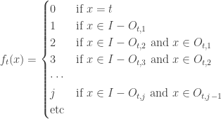
The four examples of continuous functions shown above are excellent examples to illustrate the Sorgenfrey topology. We now introduce a family of continuous functions $f_a:\mathbb{S} \rightarrow \mathbb{R}$ for $0<a<1$ . These continuous functions will lead to additional insight on the function space whose domain space is the Sorgenfrey line.

For any $0<a<1$ , the following gives the definition and the graph of the function $f_a$ .

$\displaystyle f_a(x) = \left\{ \begin{array}{ll} \displaystyle 0 &\ \ \ \ \ \ -\infty<x<-1 \\ \text{ } & \text{ } \\ \displaystyle 1 &\ \ \ \ \ \ -1 \le x<-a \\ \text{ } & \text{ } \\ 0 &\ \ \ \ \ \ -a \le x <a \\ \text{ } & \text{ } \\ 1 &\ \ \ \ \ \ a \le x <1 \\ \text{ } & \text{ } \\ 0 &\ \ \ \ \ \ 1 \le x <\infty \end{array} \right.$

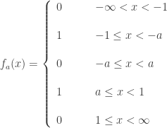
Figure 5 – a family of Sorgenfrey continuous functions

Function Space on the Sorgenfrey Line

This is the place where we switch the focus to function space. The set $C(\mathbb{S})$ is a subset of the product space $\mathbb{R}^\mathbb{R}$ . So we can consider $C(\mathbb{S})$ as a topological space endowed with the topology inherited as a subspace of $\mathbb{R}^\mathbb{R}$ . This topology on $C(\mathbb{S})$ is called the pointwise convergence topology and $C(\mathbb{S})$ with the product subspace topology is denoted by $C_p(\mathbb{S})$ . See here for comments on how to work with the pointwise convergence topology.

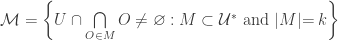
For the present discussion, all we need is some notation on a base for $C_p(\mathbb{S})$ . For $x \in \mathbb{S}$ , and for any open interval $(a,b)$ (open in the usual topology of the real number line), let $[x,(a,b)]=\left\{h \in C_p(\mathbb{S}): h(x) \in (a, b) \right\}$ . Then the collection of intersections of finitely many $[x,(a,b)]$ would form a base for $C_p(\mathbb{S})$ .

The following is the main fact we wish to establish.

The function space $C_p(\mathbb{S})$ contains a closed and discrete subspace of cardinality continuum. In particular, the set $F=\left\{f_a: 0<a<1 \right\}$ is a closed and discrete subspace of $C_p(\mathbb{S})$ .

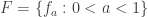
The above result will derive several facts on the function space $C_p(\mathbb{S})$ , which are discussed in a section below. More interestingly, the proof of the fact that $F=\left\{f_a: 0<a<1 \right\}$ is a closed and discrete subspace of $C_p(\mathbb{S})$ is based purely on the definition of the functions $f_a$ and the Sorgenfrey topology. The proof given below does not use any deep or high powered results from function space theory. So it should be a nice exercise on the Sorgenfrey topology.

I invite readers to either verify the fact independently of the proof given here or follow the proof closely. Lots of drawing of the functions $f_a$ on paper will be helpful in going over the proof. In this one instance at least, drawing continuous functions can help gain insight on function spaces.

Working out the Proof

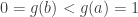
The following diagram was helpful to me as I worked out the different cases in showing the discreteness of the family $F=\left\{f_a: 0<a<1 \right\}$ . The diagram is a valuable aid in convincing myself that a given case is correct.

Figure 6 – A comparison of three Sorgenfrey continuous functions

Now the proof. First, $F$ is relatively discrete in $C_p(\mathbb{S})$ . We show that for each $a$ , there is an open set $O$ containing $f_a$ such that $O$ does not contain $f_w$ for any $w \ne a$ . To this end, let $O=[a,V_1] \cap [-a,V_2]$ where $V_1$ and $V_2$ are the open intervals $V_1=(0.9,1.1)$ and $V_2=(-0.1,0.1)$ . With Figure 6 as an aid, it follows that for $0<b<a$ , $f_b \notin O$ and for $a<c<1$ , $f_c \notin O$ .

The open set $O=[a,V_1] \cap [-a,V_2]$ contains $f_a$ , the function in the middle of Figure 6. Note that for $0<b<a$ , $f_b(-a)=1$ and $f_b(-a) \notin V_2$ . Thus $f_b \notin O$ . On the other hand, for $a<c<1$ , $f_c(a)=0$ and $f_c(a) \notin V_1$ . Thus $f_c \notin O$ . This proves that the set $F$ is a discrete subspace of $C_p(\mathbb{S})$ relative to $F$ itself.

Now we show that $F$ is closed in $C_p(\mathbb{S})$ . To this end, we show that

$g \in C_p(\mathbb{S})$

$U$

$g$

$U$

$F$

Actually, this has already been done above with points $g$ that are in $F$ . One thing to point out is that the range of $f_a$ is $\left\{0,1 \right\}$ . As we consider $g \in C_p(\mathbb{S})$ , we only need to consider $g$ that maps into $\left\{0,1 \right\}$ . Let $g \in C_p(\mathbb{S})$ . The argument is given in two cases regarding the function $g$ .

Case 1. There exists some $a \in (0,1)$ such that $g(a) \ne g(-a)$ .

We assume that $g(a)=0$ and $g(-a)=1$ . Then for all $0<b<a$ , $f_b(a)=1$ and for all $a<c<1$ , $f_c(-a)=0$ . Let $U=[a,(-0.1,0.1)] \cap [-a,(0.9,1.1)]$ . Then $g \in U$ and $U$ contains no $f_b$ for any $0<b<a$ and $f_c$ for any $a<c<1$ . To help see this argument, use Figure 6 as a guide. The case that $g(a)=1$ and $g(-a)=0$ has a similar argument.

Case 2. For every $a \in (0,1)$ , we have $g(a) = g(-a)$ .

Claim. The function $g$ is constant on the interval $(-1,1)$ . Suppose not. Let $0<b<a<1$ such that $g(a) \ne g(b)$ . Suppose that $0=g(b) < g(a)=1$ . Consider $W=\left\{w<a: g(w)=0 \right\}$ . Clearly the number $a$ is an upper bound of $W$ . Let $u \le a$ be a least upper bound of $W$ . The function $g$ has value 1 on the interval $(u,a)$ . Otherwise, $u$ would not be the least upper bound of the set $W$ . There is a sequence of points $\left\{x_n \right\}$ in the interval $(b,u)$ such that $x_n \rightarrow u$ from the left such that $g(x_n)=0$ for all $n$ . Otherwise, $u$ would not be the least upper bound of the set $W$ .

It follows that $g(u)=1$ . Otherwise, the function $g$ is not continuous at $u$ . Now consider the 6 points $-a<-u<-b<b<u<a$ . By the assumption in Case 2, $g(u)=g(-u)=1$ and $g(b)=g(-b)=0$ . Since $g(x_n)=0$ for all $n$ , $g(-x_n)=0$ for all $n$ . Note that $-x_n \rightarrow -u$ from the right. Since $g$ is right continuous, $g(-u)=0$ , contradicting $g(-u)=1$ . Thus we cannot have $0=g(b) < g(a)=1$ .

Now suppose we have $1=g(b) > g(a)=0$ where $0<b<a<1$ . Consider $W=\left\{w<a: g(w)=1 \right\}$ . Clearly $W$ has an upper bound, namely the number $a$ . Let $u \le a$ be a least upper bound of $W$ . The function $g$ has value 0 on the interval $(u,a)$ . Otherwise, $u$ would not be the least upper bound of the set $W$ . There is a sequence of points $\left\{x_n \right\}$ in the interval $(b,u)$ such that $x_n \rightarrow u$ from the left such that $g(x_n)=1$ for all $n$ . Otherwise, $u$ would not be the least upper bound of the set $W$ .

It follows that $g(u)=0$ . Otherwise, the function $g$ is not continuous at $u$ . Now consider the 6 points $-a<-u<-b<b<u<a$ . By the assumption in Case 2, $g(u)=g(-u)=0$ and $g(b)=g(-b)=1$ . Since $g(x_n)=1$ for all $n$ , $g(-x_n)=1$ for all $n$ . Note that $-x_n \rightarrow -u$ from the right. Since $g$ is right continuous, $g(-u)=1$ , contradicting $g(-u)=0$ . Thus we cannot have $1=g(b) > g(a)=0$ .

The claim that the function $g$ is constant on the interval $(-1,1)$ is established. To wrap up, first assume that the function $g$ is 1 on the interval $(-1,1)$ . Let $U=[0,(0.9,1.1)]$ . It is clear that $g \in U$ . It is also clear from Figure 5 that $U$ contains no $f_a$ . Now assume that the function $g$ is 0 on the interval $(-1,1)$ . Since $g$ is Sorgenfrey continuous, it follows that $g(-1)=0$ . Let $U=[-1,(-0.1,0.1)]$ . It is clear that $g \in U$ . It is also clear from Figure 5 that $U$ contains no $f_a$ .

We have established that the set $F=\left\{f_a: 0<a<1 \right\}$ is a closed and discrete subspace of $C_p(\mathbb{S})$ .

What does it Mean?

The above argument shows that the set $F$ is a closed an discrete subspace of the function space $C_p(\mathbb{S})$ . We have the following three facts.

Three Results

$C_p(\mathbb{S})$ is separable.
$C_p(\mathbb{S})$ is not hereditarily separable.
$C_p(\mathbb{S})$ is not a normal space.

To show that $C_p(\mathbb{S})$ is separable, let’s look at one basic helpful fact on $C_p(X)$ . If $X$ is a separable metric space, e.g. $X=\mathbb{R}$ , then $C_p(X)$ has quite a few nice properties (discussed here). One is that $C_p(X)$ is hereditarily separable. Thus $C_p(\mathbb{R})$ , the space of real-valued continuous functions defined on the number line with the pointwise convergence topology, is hereditarily separable and thus separable. Recall that continuous functions in $C_p(\mathbb{R})$ are also Soregenfrey line continuous. Thus $C_p(\mathbb{R})$ is a subspace of $C_p(\mathbb{S})$ . The space $C_p(\mathbb{R})$ is also a dense subspace of $C_p(\mathbb{S})$ . Thus the space $C_p(\mathbb{S})$ contains a dense separable subspace. It means that $C_p(\mathbb{S})$ is separable.

Secondly, $C_p(\mathbb{S})$ is not hereditarily separable since the subspace $F=\left\{f_a: 0<a<1 \right\}$ is a closed and discrete subspace.

Thirdly, $C_p(\mathbb{S})$ is not a normal space. According to Jones’ lemma, any separable space with a closed and discrete subspace of cardinality of continuum is not a normal space (see Corollary 1 here). The subspace $F=\left\{f_a: 0<a<1 \right\}$ is a closed and discrete subspace of the separable space $C_p(\mathbb{S})$ . Thus $C_p(\mathbb{S})$ is not normal.

Remarks

The topology of the Sorgenfrey line is vastly different from the usual topology on the real line even though the the Sorgenfrey topology is obtained by a seemingly small tweak from the usual topology. The real line is a metric space while the Sorgenfrey line is not metrizable. The real number line is connected while the Sorgenfrey line is not. The countable power of the real number line is a metric space and thus a normal space. On the other hand, the Sorgenfrey line is a classic example of a normal space whose square is not normal. See here for a basic discussion of the Sorgenfrey line.

The pictures of Sorgenfrey continuous functions demonstrated here show that the real number line and the Sorgenfrey line are also very different from a function space perspective. The function space $C_p(\mathbb{R})$ has a whole host of nice properties: normal, Lindelof (hence paracompact and collectionwise normal), hereditarily Lindelof (hence hereditarily normal), hereditarily separable, and perfectly normal (discussed here).

Though separable, the function space $C_p(\mathbb{S})$ contains a closed and discrete subspace of cardinality continuum, making it not hereditarily separable and not normal.

For more information about $C_p(X)$ in general and $C_p(\mathbb{S})$ in particular, see [1] and [2]. A different proof that $C_p(\mathbb{S})$ contains a closed and discrete subspace of cardinality continuum can be found in Problem 165 in [2].

The next post is a continuation on the theme of drawing Sorgenfrey continuous functions.

Reference

Arkhangelskii, A. V., Topological Function Spaces, Mathematics and Its Applications Series, Kluwer Academic Publishers, Dordrecht, 1992.
Tkachuk V. V., A $C_p$ -Theory Problem Book, Topological and Function Spaces, Springer, New York, 2011.

$\text{ }$

$\copyright$ 2017 – Dan Ma

A strategy for finding CCC and non-separable spaces

Posted on November 18, 2016 by Dan Ma

In this post we present a general strategy for finding CCC spaces that are not separable. As illustration, we give four implementations of this strategy.

In searching for counterexamples in topology, one good place to look is of course the book by Steen and Seebach [2]. There are four examples of spaces that are CCC but not separable found in [2] – counterexamples 20, 21, 24 and 63. Counterexamples 20 and 21 are not Hausdorff. Counterexample 24 is the uncountable Fort space (it is completely normal but not perfectly normal). Counterexample 63 (Countable Complement Extension Topology) is Hausdorff but is not regular. These are valuable examples especially the last two (24 and 63). The examples discussed below expand the offerings in Steen and Seebach.

The discussion of CCC but not separable in this post does not use axioms beyond the usual axioms of set theory (i.e. ZFC). The discussion here does not touch on Suslin lines or other examples that require extra set theory. The existence of Suslin lines is independent of ZFC. A Suslin line would produce an example of a perfectly normal first countable CCC non-separable space. In models of set theory where Suslin lines do not exist, a perfectly normal first countable CCC non-separable space can also be produced using other set-theoretic assumptions. The examples discussed below are not as nice as the set-theoretic examples since they usually are not first countable and perfectly normal.

____________________________________________________________________

The countable chain conditon

A topological space $X$ is said to have the countable chain condition (to have the CCC for short) if $\mathcal{U}$ is a disjoint collection of non-empty open subsets of $X$ (meaning that for any $A,B \in \mathcal{U}$ with $A \ne B$ , we have $A \cap B=\varnothing$ ), then $\mathcal{U}$ is countable. In other words, in a space with the CCC, there cannot be uncountably many pairwise disjoint non-empty open sets. For ease of discussion, if $X$ has the CCC, we also say that $X$ is a CCC space or X is CCC. A space $X$ is separable if there exists a countable subset $A$ of $X$ such that $A$ is dense in $X$ (meaning that if $U$ is a nonempty open subset of $X$ , then $U \cap A \ne \varnothing$ ).

It is clear that any separable space has the CCC. In metric spaces, these two properties are equivalent. Among topological spaces in general, the two properties are not identical. Thus “CCC but not separable” is one way to distinguish between metrizable spaces and non-metrizable spaces. Even in non-metrizable spaces, “CCC but not separable” is also a way to obtain more information about the spaces being investigated.

____________________________________________________________________

The strategy

Here’s the strategy for finding CCC and not separable.

Any dense subspace of a CCC space always has the CCC. Thus the search focuses on the subspaces in a CCC space that are reliably CCC. The strategy is to find non-separable spaces among these dense subspaces. The search is given an assist if the space or class of spaces in question has a characteristic that delineate the “separable” from the CCC (see Example 3 and Example 4 below).

In the following sections, we illustrate four different ways to apply the strategy.

____________________________________________________________________

Example 1

The first way is a standard example found in the literature. The space to start from is the product space of separable spaces, which is always CCC. By a theorem of Ross and Stone, the product of more than continuum many separable spaces is not separable. Thus one way to get an example of CCC but not separable space is to take the product of more than continuum many separable spaces. For example, if $c$ is the cardinality of continuum, then consider $\left\{0,1 \right\}^{2^c}$ , the product of $2^c$ many copies of $\left\{0,1 \right\}$ , or consider $X^{2^c}$ where $X$ is your favorite separable space.

____________________________________________________________________

Example 2

The second implementation of the strategy is also from taking the product of separable spaces. This time the number of factors does not have to be more than continuum. Here, we focus on one particular dense subspace of the product space, the $\Sigma$ -products. To make this clear, let’s focus on a specific example. Consider $X=\left\{0,1 \right\}^{c}$ where $c$ is the cardinality of continuum. Consider the following subspace.

$\Sigma(\left\{0,1 \right\}^{c})= \left\{x \in X: x(\alpha) \ne 0 \text{ for at most countably many } \alpha < c \right\}$

The subspace $\Sigma(\left\{0,1 \right\}^{c})$ is dense in $X$ , thus has CCC. It is straightforward to verify that $\Sigma(\left\{0,1 \right\}^{c})$ is not separable.

To implement this example, find any space $X$ which is a product space of separable spaces, each of which has at least two point (one of the points is labeled 0). The dense subspace is the $\Sigma$ -product, which is the subspace consisting of all points that are non-zero at only countably many coordinates. The $\Sigma$ -product has the countable chain condition since it is a dense subspace of the CCC space $X$ . The $\Sigma$ -product is not separable since there are uncountably many factors in the product space $X$ and that each factor has at least two points. This idea had been implemented in this previous post.

____________________________________________________________________

Example 3

The third class of spaces is the class of Pixley-Roy spaces, which are hyperspaces. Given a space $X$ , let $\mathcal{F}[X]$ be the set of all non-empty finite subsets of $X$ . For $F \in \mathcal{F}[X]$ and for any open subset $U$ of $X$ , let $[F,U]=\left\{B \in \mathcal{F}[X]: F \subset B \subset U \right\}$ . The sets $[F,U]$ over all $F$ and $U$ form a base for a topology on $\mathcal{F}[X]$ . This topology is called the Pixley-Roy topology (or Pixley-Roy hyperspace topology). The set $\mathcal{F}[X]$ with this topology is called a Pixley-Roy space.

The Pixley-Roy hyperspaces are discussed in this previous post. Whenever the ground space $X$ is uncountable, $\mathcal{F}[X]$ is not a separable space. We need to identify the $\mathcal{F}[X]$ that are CCC. According to the previous post on Pixley-Roy hyperspaces, for any space $X$ with a countable network, $\mathcal{F}[X]$ is CCC. Thus for any uncountable space $X$ with a countable network, the Pixley-Roy space $\mathcal{F}[X]$ is a CCC space that is not separable. The following gives a few such examples.

$\mathcal{F}[\mathbb{R}]$

$\mathcal{F}[X]$ where $X$ is any uncountable, separable and metrizable space.

$\mathcal{F}[X]$ where $X$ is uncountable and is the continuous image of a separable metrizable space.

Spaces with countable networks are discussed in this previous post. An example of a space $X$ that is the continuous image of a separable metrizable space is the bow-tie space found this previous post. Another example is any quote space of a separable metrizable space.

____________________________________________________________________

Example 4

For the fourth implementation of the strategy, we go back to the product space of separable spaces in Example 2, with the exception that the focus is on the product of the real line $\mathbb{R}$ . Let $X$ be any uncountable completely regular space. The product space $\mathbb{R}^X$ always has the CCC since it is a product of separable space. Now we single out a dense subspace of $\mathbb{R}^X$ for which there is a characterization for separability, namely the subspace $C(X)$ , which is the set of all continuous functions from $X$ into $\mathbb{R}$ . The subspace $C(X)$ as a topological space is usually denoted by $C_p(X)$ . For a basic discussion of $C_p(X)$ , see this previous post.

We know precisely when $C_p(X)$ is separable. The following theorem captures the idea.

Theorem 1 – Theorem I.1.3 [1]
The function space $C_p(X)$ is separable if and only if the domain space $X$ has a weaker (or coarser) separable metric topology (in other words, $X$ is submetrizable with a separable metric topology).

Based on the theorem, $C_p(X)$ is separable for any separable metric space $X$ . Other examples of separable $C_p(X)$ include spaces $X$ that are created by tweaking the usual Euclidean topology on the real line and at the same time retaining the usual real line topology as a weaker topology, e.g. the Sorgenfrey line and the Michael line. Thus $C_p(X)$ would be separable if $X$ is a space such as the Sorgenfrey line or the Michael line. For our purpose at hand, we need to look for spaces that are not like the Sorgenfrey line or the Michael line. Here’s some examples of spaces $X$ that have no weaker separable metric topology.

Any compact space $X$ that is not metrizable.
The space $X=\omega_1$ , the first uncountable ordinal with the order topology.
Any space $X=C_p(Y)$ where $Y$ is not separable.

The function space $C_p(X)$ for any one of the above three spaces has the CCC but is not separable. It is well known that any compact space with a weaker metrizable topology is metrizable. Some examples for compact $X$ are: the first uncountable successor ordinal $\omega_1+1$ , the double arrow space, and the product space $\left\{0,1 \right\}^{\omega_1}$ .

It can be shown that $C_p(\omega_1)$ is not separable (see this previous post). The last example is due to the following theorem.

Theorem 2 – Theorem I.1.4 [1]
The function space $C_p(Y)$ has a weaker (or coarser) separable metric topology if and only if the domain space $Y$ is separable.

Thus picking a non-separable space $Y$ would guarantee that $C_p(Y)$ has no weaker separable metric topology. As a result, $C_p(C_p(Y))$ is a CCC and not separable space.

Interestingly, Theorem 1 and Theorem 2 show a duality existing between the property of having a weaker separable metric topology and the property of being separable. The two theorems allow us to switch the two properties between the domain space and the function space.

____________________________________________________________________

Remarks

Another interesting point to make is that Theorem 1 and Theorem 2 together allow us to “buy one get one free.” Once we obtain a space $X$ that is CCC and not separable from any one of the avenues discussed here, the function space $C_p(X)$ has no weaker separable metric topology (by Theorem 2) and the function space $C_p(C_p(X))$ is another example of CCC and not separable.

The strategy discussed above unifies all four examples. Undoubtedly there will be other examples that can come from the strategy. To find more examples, find a space or a class of spaces that are reliably CCC and then look for potential non-separable spaces among the dense subspaces of the starting space.

____________________________________________________________________

Exercises

Show that in metrizable spaces, CCC and separable are equivalent. The only part that needs to be shown is that if $X$ is metrizable and CCC, then $X$ is separable.
Show that any dense subspace of a CCC space is also CCC.
Verify that the space $\Sigma(\left\{0,1 \right\}^{c})$ defined in Example 2 is dense in $X$ and is not separable.
Verify that the Pixley-Roy space $\mathcal{F}[\mathbb{R}]$ defined in Example 3 is CCC and not separable.
Verify that function space $C_p(\omega_1)$ mentioned in Example 4 is not separable. Hint: use the pressing down lemma.

____________________________________________________________________

Reference

Arkhangelskii, A. V., Topological Function Spaces, Mathematics and Its Applications Series, Kluwer Academic Publishers, Dordrecht, 1992.
Steen, L. A., Seebach, J. A., Counterexamples in Topology, Dover Publications, Inc., New York, 1995.

____________________________________________________________________
$\copyright \ 2016 \text{ by Dan Ma}$
Revised October 26, 2018

Cp(X) where X is a separable metric space

Posted on April 3, 2014 by Dan Ma

Let $\tau$ be an uncountable cardinal. Let $\prod_{\alpha < \tau} \mathbb{R}=\mathbb{R}^{\tau}$ be the Cartesian product of $\tau$ many copies of the real line. This product space is not normal since it contains $\prod_{\alpha \in \omega_1} \omega=\omega^{\omega_1}$ as a closed subspace. However, there are dense subspaces of $\mathbb{R}^{\tau}$ are normal. For example, the $\Sigma$ -product of $\tau$ copies of the real line is normal, i.e., the subspace of $\mathbb{R}^{\tau}$ consisting of points which have at most countably many non-zero coordinates (see this post). In this post, we look for more normal spaces among the subspaces of $\mathbb{R}^{\tau}$ that are function spaces. In particular, we look at spaces of continuous real-valued functions defined on a separable metrizable space, i.e., the function space $C_p(X)$ where $X$ is a separable metrizable space.

For definitions of basic open sets and other background information on the function space $C_p(X)$ , see this previous post.

____________________________________________________________________

$C_p(X)$ when $X$ is a separable metric space

In the remainder of the post, $X$ denotes a separable metrizable space. Then, $C_p(X)$ is more than normal. The function space $C_p(X)$ has the following properties:

normal,
Lindelof (hence paracompact and collectionwise normal),
hereditarily Lindelof (hence hereditarily normal),
hereditarily separable,
perfectly normal.

All such properties stem from the fact that $C_p(X)$ has a countable network whenever $X$ is a separable metrizable space.

Let $L$ be a topological space. A collection $\mathcal{N}$ of subsets of $L$ is said to be a network for $L$ if for each $x \in L$ and for each open $O \subset L$ with $x \in O$ , there exists some $A \in \mathcal{N}$ such that $x \in A \subset O$ . A countable network is a network that has only countably many elements. The property of having a countable network is a very strong property, e.g., having all the properties listed above. For a basic discussion of this property, see this previous post and this previous post.

To define a countable network for $C_p(X)$ , let $\mathcal{B}$ be a countable base for the domain space $X$ . For each $B \subset \mathcal{B}$ and for any open interval $(a,b)$ in the real line with rational endpoints, consider the following set:

$[B,(a,b)]=\left\{f \in C(X): f(B) \subset (a,b) \right\}$

There are only countably many sets of the form $[B,(a,b)]$ . Let $\mathcal{N}$ be the collection of sets, each of which is the intersection of finitely many sets of the form $[B,(a,b)]$ . Then $\mathcal{N}$ is a network for the function space $C_p(X)$ . To see this, let $f \in O$ where $O=\bigcap_{x \in F} [x,O_x]$ is a basic open set in $C_p(X)$ where $F \subset X$ is finite and each $O_x$ is an open interval with rational endpoints. For each point $x \in F$ , choose $B_x \in \mathcal{B}$ with $x \in B_x$ such that $f(B_x) \subset O_x$ . Clearly $f \in \bigcap_{x \in F} \ [B_x,O_x]$ . It follows that $\bigcap_{x \in F} \ [B_x,O_x] \subset O$ .

Examples include $C_p(\mathbb{R})$ , $C_p([0,1])$ and $C_p(\mathbb{R}^\omega)$ . All three can be considered subspaces of the product space $\mathbb{R}^c$ where $c$ is the cardinality of the continuum. This is true for any separable metrizable $X$ . Note that any separable metrizable $X$ can be embedded in the product space $\mathbb{R}^\omega$ . The product space $\mathbb{R}^\omega$ has cardinality $c$ . Thus the cardinality of any separable metrizable space $X$ is at most continuum. So $C_p(X)$ is the subspace of a product space of $\le$ continuum many copies of the real lines, hence can be regarded as a subspace of $\mathbb{R}^c$ .

A space $L$ has countable extent if every closed and discrete subset of $L$ is countable. The $\Sigma$ -product $\Sigma_{\alpha \in A} X_\alpha$ of the separable metric spaces $\left\{X_\alpha: \alpha \in A \right\}$ is a dense and normal subspace of the product space $\prod_{\alpha \in A} X_\alpha$ . The normal space $\Sigma_{\alpha \in A} X_\alpha$ has countable extent (hence collectionwise normal). The examples of $C_p(X)$ discussed here are Lindelof and hence have countable extent. Many, though not all, dense normal subspaces of products of separable metric spaces have countable extent. For a dense normal subspace of a product of separable metric spaces, one interesting problem is to find out whether it has countable extent.

____________________________________________________________________

$\copyright \ 2014 \text{ by Dan Ma}$

Working with the function space Cp(X)

Posted on April 3, 2014 by Dan Ma

This post provides basic information about the space of real-valued continuous functions with the pointwise convergence topology. The goal is to discuss the setting and to define the standard basic open sets in the function space, providing background information for subsequent posts.

____________________________________________________________________

Completely Regular Spaces

The starting point is a completely regular space. A space $X$ is said to be completely regular if $X$ is a $T_0$ space and for each $x \in X$ and for each closed subset $A$ of $X$ with $x \notin A$ , there is a continuous function $f:X \rightarrow [0,1]$ such that $f(A) \subset \left\{0 \right\}$ and $f(x)=1$ . Note that the $T_0$ axiom and the existence of the continuous function imply the $T_1$ axiom, which is equivalent to the property that single points are closed sets. Completely regular spaces are also called Tychonoff spaces.

____________________________________________________________________

Defining the Function Space $C_p(X)$

Let $X$ be a completely regular space. Let $C(X)$ be the set of all real-valued continuous functions defined on the space $X$ . The set $C(X)$ is naturally a subspace of the product space $\prod_{x \in X} \mathbb{R}=\mathbb{R}^X$ . Thus $C(X)$ can be endowed with the subspace topology inherited from the product space $\mathbb{R}^X$ . When this is the case, the function space $C(X)$ is denoted by $C_p(X)$ . The topology on $C_p(X)$ is called the pointwise convergence topology.

Now we need a good handle on the open sets in the function space $C_p(X)$ . A basic open set in the product space $\mathbb{R}^X$ is of the form $\prod_{x \in X} U_x$ where each $U_x$ is an open subset of $\mathbb{R}$ such that $U_x = \mathbb{R}$ for all but finitely many $x \in X$ (equivalently $U_x \ne \mathbb{R}$ for only finitely many $x \in X$ ). Thus a basic open set in $C_p(X)$ is of the form:

$C(X) \cap \biggl(\prod_{x \in X} U_x \biggr) \ \ \ \ \ \ \ \ \ \ \ \ \ \ \ \ \ \ \ \ \ \ \ \ \ \ \ \ (1)$

where each $U_x$ is an open subset of $\mathbb{R}$ and $U_x = \mathbb{R}$ for all but finitely many $x \in X$ . In addition, when $U_x \ne \mathbb{R}$ , we can take $U_x$ to be an open interval of the form $(a,b)$ . To simplify notation, the basic open sets as described in (1) can also be notated by:

$\prod_{x \in X} U_x \ \ \ \ \ \ \ \ \ \ \ \ \ \ \ \ \ \ \ \ \ \ \ \ \ \ \ \ \ \ \ \ \ \ \ \ \ \ \ \ \ \ (1a)$

Thus when working with open sets in $C_p(X)$ , we take $\prod_{x \in X} U_x$ to mean the set of all $f \in C(X)$ such that $f(x) \in U_x$ for each $x \in X$ .

To make the basic open sets of $C_p(X)$ more explicit, (1) or (1a) is translated as follows:

$\bigcap_{x \in F} \ [x, O_x] \ \ \ \ \ \ \ \ \ \ \ \ \ \ \ \ \ \ \ \ \ \ \ \ \ \ \ \ \ \ \ \ \ \ \ \ \ \ (2)$

where $F \subset X$ is a finite set, for each $x \in F$ , $O_x$ is an open interval of $\mathbb{R}$ , and $[x,O_x]$ is the set of all $f \in C(X)$ such that $f(x) \in O_x$ .

There is another description of basic open sets that is useful. Let $f \in C_p(X)$ . Let $F \subset X$ be finite. Let $\epsilon>0$ . Let $B(f,F,\epsilon)$ be defined as follows:

$B(f,F,\epsilon)=\left\{g \in C(X): \forall \ x \in F, \lvert f(x)-g(x) \lvert< \epsilon \right\} \ \ \ \ \ \ \ (3)$

In proving results about $C_p(X)$ , we can use basic open sets that are described in any one of the three forms (1), (2) and (3). If $U$ is a basic open subset of $C_p(X)$ , as described in (1) or (1a), we use $supp(U)$ to denote the finite set of $x \in X$ such that $U_x \ne \mathbb{R}$ . The set $supp(U)$ is called the support of $U$ . The support for the basic open sets as described in (2) and (3) is already explicitly stated.

____________________________________________________________________

Basic Discussion

The theory of $C_p(X)$ is a vast subject area. For a systematic introduction, see [1]. One fundamental theme in function space theory is the study of how properties of $X$ and $C_p(X)$ are related. The domain space $X$ and the function space $C(X)$ are not on the same footing. The domain $X$ only has a topological structure. The function space $C_p(X)$ carries a topology and two natural algebraic operations of addition and multiplication, making it a topological ring. In addition, $C_p(X)$ can be regarded as a topological group, or a linear topological space. In this post and in many subsequent posts, we narrow the focus to the topological properties of $X$ and $C_p(X)$ , paying attention to the how the topological properties of $X$ and $C_p(X)$ are related.

In addition to the pointwise convergence topology, there are other topologies that can be defined on $C(X)$ , e.g., the compact-open topology, the topology of uniform convergence and others. Both the pointwise convergence topology and the compact-open topology are examples of set-open topologies. In this post and in many of the subsequent posts, the focus is on the pointwise convergence topology, i.e., the subspace topology on $C(X)$ inherited from the product space.

The space $C_p(X)$ automatically inherits certain properties of the product space $\mathbb{R}^X$ . Note that $C(X)$ is dense in $\mathbb{R}^X$ . The product $\mathbb{R}^X$ has the countable chain condition (CCC) since it is a product of separable spaces. Hence $C_p(X)$ always has the CCC, i.e., there are no uncountably many pairwise disjoint open subsets of $C_p(X)$ , regardless what the domain space $X$ is. One consequence of the CCC is that $C_p(X)$ is paracompact if and only if $C_p(X)$ is Lindelof.

It is well known that $\mathbb{R}^X$ is separable if and only if the cardinality of $X$ $\le$ continuum. Since $C(X)$ is dense in $\mathbb{R}^X$ , $C_p(X)$ is not separable if the cardinality of $X$ $>$ continuum. Thus $C_p(X)$ is one way to get a CCC space that is not separable. There are non-separable $C_p(X)$ where the cardinality of $X$ $\le$ continuum. Obtaining such $C_p(X)$ would require more than the properties of the product space $\mathbb{R}^X$ ; using properties of $X$ would be necessary.

The properties of $C_p(X)$ discussed so far are inherited from the product space. Refer to chapter one of [1] for other elementary properties of $C_p(X)$ . See this post for a discussion of $C_p(X)$ where $X$ is a separable metric space. See this post about a consequence of normality of $C_p(X)$ .

____________________________________________________________________

Reference

Arkhangelskii, A. V., Topological Function Spaces, Mathematics and Its Applications Series, Kluwer Academic Publishers, Dordrecht, 1992.

____________________________________________________________________

$\copyright \ 2014 \text{ by Dan Ma}$

A factorization theorem for products of separable spaces

Posted on March 23, 2014 by Dan Ma

Let $X=\prod_{\alpha \in A} X_\alpha$ be a product space. Let $f:X \rightarrow T$ be a continuous function where $T$ is a topological space. In this post, we discuss what it means for the continuous function $f$ to depend on countably many coordinates and then discuss some conditions that we can impose on the product space and on the range space $T$ to ensure that every continuous $f$ defined on the product space will depend on countably many coordinates. This notion of a continuous function depending on countably many coordinates is equivalent to factoring the continuous function into the composition of a projection map and a continuous function defined on a countable subproduct (see Lemma 1 below).

Let’s set some notation about the product space we work with in this post. Let $X=\prod_{\alpha \in A} X_\alpha$ be a product space. Let $T$ be a topological space. Let $f:X \rightarrow T$ be continuous. For any $B \subset A$ , $\pi_B$ is the natural projection from the full product space $X=\prod_{\alpha \in A} X_\alpha$ into the subproduct $\prod_{\alpha \in B} X_\alpha$ . Standard basic open sets of $X=\prod_{\alpha \in A} X_\alpha$ are of the form $\prod_{\alpha \in A} O_\alpha$ where each $O_\alpha$ is open in $X_\alpha$ and that $O_\alpha=X_\alpha$ for all but finitely many $\alpha \in A$ . We use $supp(\prod_{\alpha \in A} O_\alpha)$ to denote the finite set of $\alpha \in A$ where $O_\alpha \ne X_\alpha$ .

____________________________________________________________________

Factoring a Continuous Map

The function $f$ is said to depend on countably many coordinates if there exists a countable set $B \subset A$ such that for any $x,y \in X$ , if $x_\alpha=y_\alpha$ for all $\alpha \in B$ , then $f(x)=f(y)$ . Suppose $f$ is instead defined on a subspace $Y$ of $X$ . The function $f$ is said to depend on countably many coordinates if there exists a countable $B \subset A$ such that for any $x,y \in Y$ , if $x_\alpha=y_\alpha$ for all $\alpha \in B$ , then $f(x)=f(y)$ .

We have the following lemmas.

Lemma 1

$X=\prod_{\alpha \in A} X_\alpha$

$T$

$f:X \rightarrow T$

There exists a countable $B \subset A$ such that for any $x,y \in X$ , if $x_\alpha=y_\alpha$ for all $\alpha \in B$ , then $f(x)=f(y)$ .
There exists a countable $B \subset A$ such that $f=g \circ \pi_B$ where $g: \prod_{\alpha \in B} X_\alpha \rightarrow T$ is continuous.

Lemma 1a

$X=\prod_{\alpha \in A} X_\alpha$

$T$

$Y$

$X$

$f:Y \rightarrow T$

There exists a countable $B \subset A$ such that for any $x,y \in Y$ , if $x_\alpha=y_\alpha$ for all $\alpha \in B$ , then $f(x)=f(y)$ .
There exists a countable $B \subset A$ such that $f=g \circ \pi_B$ where $g: \pi_B(Y) \rightarrow T$ is continuous.

It is straightforward to verify Lemma 1 and Lemma 1a. We use condition 1 to define what it means for a function to be dependent on countably many coordinates. Both lemmas indicate that either condition is a valid definition. These two lemmas also indicate why the notion being discussed can be called a factorization notion.

____________________________________________________________________

When a Continuous Map Can Be Factored

We discuss some conditions that we can place on the product space $X=\prod_{\alpha \in A} X_\alpha$ and on the range space $T$ so that any continuous map depends on countably many coordinates. We prove the following theorem.

Theorem 1

$X=\prod_{\alpha \in A} X_\alpha$

$X_\alpha$

$T$

$Y$

$X$

$f:Y \rightarrow T$

Before stating the main theorem, we need one more lemma. Let $W \subset X=\prod_{\alpha \in A} X_\alpha$ . The set $W$ is said to depend on countably many coordinates if there exists a countable $B \subset A$ such that for any $x \in W$ and for any $y \in X$ , if $x_\alpha=y_\alpha$ for all $\alpha \in B$ , then $y \in W$ .

When we try to determine whether a function $f:Y \rightarrow T$ , where $Y \subset X$ , can be factored, we will need to decide whether a set $W \subset Y$ depends on countably many coordinates. Let $W \subset Y \subset X=\prod_{\alpha \in A} X_\alpha$ . The set $W$ is said to depend on countably many coordinates if there exists a countable $B \subset A$ such that for any $x \in W$ and for any $y \in Y$ , if $x_\alpha=y_\alpha$ for all $\alpha \in B$ , then $y \in W$ . We have the following lemma.

Lemma 2

$X=\prod_{\alpha \in A} X_\alpha$

$Y$

$X$

Let $U$ be an open subset of $X$ . Then $\overline{U}$ depends on countably many coordinates.
Let $W$ be an open subset of $Y$ . Then $\overline{W}$ depends on countably many coordinates (closure in $Y$ ).

Proof of Lemma 2
Proof of Part 1
Let $U \subset X$ be open. Let $\mathcal{B}$ be a collection of pairwise disjoint open subsets of the open set $U \subset X$ such that $\mathcal{B}$ is maximal with this property, i.e., if you throw one more open set into $\mathcal{B}$ , it will be no longer pairwise disjoint. Let $V=\bigcup \mathcal{B}$ . Since $\mathcal{B}$ is maximal, $\overline{V}=\overline{U}$ . Since $X$ has the countable chain condition, $\mathcal{B}$ is countable.

Let $B=\bigcup \left\{supp(O): O \in \mathcal{B} \right\}$ . The set $B$ is a countable subset of $A$ since $B$ is the union of countably many finite sets. We have the following claims.

Claim 1
The open set $V$ depends on the coordinates in $B$ .

Let $x \in V$ and $y \in X$ such that $x_\alpha=y_\alpha$ for all $\alpha \in B$ . We need to show that $y \in V$ . Firstly, $x \in O$ for some $O \in \mathcal{B}$ . It follows that $x_\alpha=y_\alpha$ for all $\alpha \in supp(O)$ . Thus $y \in O \subset V$ . This completes the proof of Claim 1.

Claim 2
The set $\overline{V}$ depends on the coordinates in $B$ .

Let $x \in \overline{V}$ and $y \in X$ such that $x_\alpha=y_\alpha$ for all $\alpha \in B$ . We need to show $y \in \overline{V}$ . To this end, let $O=\prod_{\alpha \in A} O_\alpha$ be a standard basic open set with $y \in O$ . The goal is to find some $q \in O \cap V$ . Define $G=\prod_{\alpha \in A} G_\alpha$ such that $G_\alpha=O_\alpha$ for all $\alpha \in B$ and $G_\alpha=X_\alpha$ for all $\alpha \in A-B$ . Then $x \in G$ . Since $x \in \overline{V}$ , there exists some $p \in V \cap G$ . Define $q$ such that $q_\alpha=p_\alpha$ for all $\alpha \in B$ and $q_\alpha=y_\alpha$ for all $\alpha \in A-B$ . Since $supp(V) \subset B$ , $q \in V$ . On the other hand, $q \in O$ . This completes the proof of Claim 2.

As noted above, $\overline{V}=\overline{U}$ . Thus $\overline{U}$ depends on countably many coordinates, namely the coordinates in the set $B$ . This completes the proof of Part 1.

Proof of Part 2
For any $S \subset X$ , let $\overline{S}$ denote the closure of $S$ in $Y$ . Let $Cl_X(S)$ denote the closure of $S$ in $X$ . Let $W \subset Y$ be open. Let $W_1$ be open in $X$ such that $W=W_1 \cap Y$ . By Part 1, $Cl_X(W_1)$ depends on countably many coordinates, say the coordinates in the countable set $B \subset A$ . This means that for any $x \in Cl_X(W_1)$ and for any $y \in X$ , if $x_\alpha=y_\alpha$ for all $\alpha \in B$ , then $y \in Cl_X(W_1)$ . Thus for any $x \in \overline{W}$ and for any $y \in Y$ , if $x_\alpha=y_\alpha$ for all $\alpha \in B$ , then $y \in Cl_X(W_1)$ . If we have $y \in \overline{W}$ , then we are done. So we only need to show that if $y \in Y$ and $y \in Cl_X(W_1)$ , then $y \in \overline{W}$ . This is why we need to assume $Y$ is dense in $X$ .

Let $y \in Y$ and $y \in Cl_X(W_1)$ . Let $C$ be an open subset of $Y$ with $y \in C$ . There exists an open subset $D$ of $X$ such that $C=D \cap Y$ . Then $D \cap Cl_X(W_1) \ne \varnothing$ . Note that $D \cap W_1$ is open and $D \cap W_1 \ne \varnothing$ . Since $Y$ is dense in $X$ , $D \cap W_1$ must contain points of $Y$ . These points of $Y$ are also points of $W$ . Thus $C$ contains points of $W$ . It follows that $y \in \overline{W}$ . This concludes the proof of Part 2. $\blacksquare$

Proof of Theorem 1
Let $Y$ be a dense subspace of $X=\prod_{\alpha \in A} X_\alpha$ . Let $f:Y \rightarrow T$ be continuous. Let $\mathcal{M}$ be a countable base for the separable metrizable space $T$ . By Lemma 2 Part 2, for each $M \in \mathcal{M}$ , $\overline{f^{-1}(M)}$ depends on countably many coordinates, say the countable set $B_M$ . Let $B=\bigcup_{M \in \mathcal{M}} B_M$ .

We claim that $B$ is a countable set of coordinates we need. Let $x,y \in Y$ such that $x_\alpha=y_\alpha$ for all $\alpha \in B$ . We need to show that $f(x)=f(y)$ . Suppose $f(x) \ne f(y)$ . Choose $\left\{M_1,M_2,M_3,\cdots \right\} \subset \mathcal{M}$ such that

$\left\{f(x) \right\}=\bigcap_{j=1}^\infty M_j=\bigcap_{j=1}^\infty \overline{M_j}$
$\overline{M_{j+1}} \subset M_j$ for each $j$

This is possible since $T$ is a second countable space. Then $f(y) \notin \overline{M_{k}}$ for some $k$ . Furthermore, $y \notin f^{-1}(\overline{M_{k}})$ . Since $f$ is continuous, $\overline{f^{-1}(M_{k})} \subset f^{-1}(\overline{M_{k}})$ . Therefore, $y \notin \overline{f^{-1}(M_{k})}$ . On the other hand, $\overline{f^{-1}(M_{k})}$ depends on the countably many coordinates in $B_{M_k}$ . We assume above that $x_\alpha=y_\alpha$ for all $\alpha \in B$ . Thus $x_\alpha=y_\alpha$ for all $\alpha \in B_{M_k}$ . This means that $y \in \overline{f^{-1}(M_{k})}$ , a contradiction. It must be that case that $f(x)=f(y)$ . $\blacksquare$

____________________________________________________________________

Another Version

We state another version of Theorem 1 that will be useful in some situations.

Theorem 2

$X=\prod_{\alpha \in A} X_\alpha$

$X_\alpha$

$T$

$Y$

$X$

$f:Y \times Y \rightarrow T$

$f$

There exists a countable set $C \subset A$ such that for any $(x,y),(p,q) \in Y \times Y$ , if $x_\alpha=p_\alpha$ and $y_\alpha=q_\alpha$ for all $\alpha \in C$ , then $f(x,y)=f(p,q)$ .
There exists a countable set $C \subset A$ and there exists a continuous $g:\pi_C(Y) \times \pi_C(Y) \rightarrow T$ such that $f=g \circ (\pi_C \times \pi_C)$ .

The map $\pi_C \times \pi_C$ is the projection map from $\prod_{\alpha \in A} X_\alpha \times \prod_{\alpha \in A} X_\alpha$ into the subproduct $\prod_{\alpha \in C} X_\alpha \times \prod_{\alpha \in B} X_\alpha$ defined by $(\pi_C \times \pi_C)(x,y)=(\pi_C(x),\pi_C(y))$ . In Theorem 2, we only need to consider $\pi_C \times \pi_C$ being defined on the subspace $Y \times Y$ .

Theorem 2 follows from Theorem 1. It is only a matter of fitting Theorem 2 in the framework of Theorem 1. Note that the product $\prod_{\alpha \in A} X_\alpha \times \prod_{\alpha \in A} X_\alpha$ is identical to the product $\prod_{\alpha \in A \cup A^*} X_\alpha$ where $A^*$ is a disjoint copy of the index set $A$ . For $(x,y) \in \prod_{\alpha \in A} X_\alpha \times \prod_{\alpha \in A} X_\alpha$ , let $x \times y \in \prod_{\alpha \in A \cup A^*} X_\alpha$ be defined by $(x \times y)_\alpha=x_\alpha$ for all $\alpha \in A$ and $(x \times y)_\alpha=y_\alpha$ for all $\alpha \in A^*$ .

With the identification of $(x,y)$ with $x \times y$ , we have a setting that fits Theorem 1. The product $\prod_{\alpha \in A \cup A^*} X_\alpha$ is also a product of separable spaces. The set $Y \times Y$ is a dense subspace of the product $\prod_{\alpha \in A \cup A^*} X_\alpha$ . In this new setting, we view a point in $Y \times Y$ as $x \times y$ . The map $f:Y \times Y \rightarrow T$ is still a continuous map. We can now apply Theorem 1.

Let $B \subset A \cup A^*$ be a countable set such that for all $x \times y,p \times q \in Y \times Y$ , if $(x \times y)_\alpha=(p \times q)_\alpha$ for all $\alpha \in B$ , then $f(x \times y)=f(p \times q)$ . Specifically, if $x_\alpha=p_\alpha$ for all $\alpha \in B \cap A$ and $y_\alpha=q_\alpha$ for all $\alpha \in B \cap A^*$ , then $f(x,y)=f(p,q)$ .

Choose a countable set $C \subset A$ such that $B \cap A \subset C$ and $B \cap A^* \subset C^*$ . Here, $C^*$ is the copy of $C$ in $A^*$ . We claim that $C$ is a countable set we need in condition 1 of Theorem 2. Let $(x,y),(p,q) \in Y \times Y$ such that $x_\alpha=p_\alpha$ and $y_\alpha=q_\alpha$ for all $\alpha \in C$ . This implies that $x_\alpha=p_\alpha$ for all $\alpha \in B \cap A$ and $y_\alpha=q_\alpha$ for all $\alpha \in B \cap A^*$ . Then $f(x,y)=f(p,q)$ . Thus condition 1 of Theorem 2 holds. It is also straightforward to verify that Condition 1 and Condition 2 are equivalent.

____________________________________________________________________

Remarks

The notion of factorizing a continuous map defined on a product space is an old topic. Theorem 1 discussed in this post is based on Theorem 4 found in [6]. Theorem 4 found in [6] is to factor continuous maps defined on a product of separable spaces. Theorem 1 in this post is modified to consider continuous maps defined on a dense subspace of a product of separable spaces. This modification will make it more useful. The references listed below represent a small sample of papers or books that have involves theorems of factoring functions defined on products. The work in [3] and [5] have more systematic treatment.

____________________________________________________________________

Reference

Brandenburg H., Husek M., On mappings from products into developable spaces, Topology Appl., 26, 229-238, 1987.
Engelking R., General Topology, Revised and Completed edition, Heldermann Verlag, Berlin, 1989.
Engelking R., On functions defined on Cartesian products, Fund. Math., 59, 221-231, 1966.
Keesling J., Normality and infinite product spaces, Adv. in. Math., 9, 90-92, 1972.
Noble N., Ulmer M., Factoring functions on Cartesian products, Trans. Amer. Math. Soc., 163, 329-339, 1972.
Ross K. A., Stone A. H., Products of separable spaces, Amer. Math. Monthly, 71, 398-403, 1964.

____________________________________________________________________

$\copyright \ 2014 \text{ by Dan Ma}$

A lemma dealing with normality in products of separable metric spaces

Posted on March 19, 2014 by Dan Ma

In this post we prove a lemma that is a great tool for working with product spaces of separable metrizable spaces. As an application of the lemma, we give an alternative proof for showing the non-normality of the product space of uncountably many copies of the discrete space of the non-negative integers.

Consider the product space $X=\prod_{\alpha \in A} X_\alpha$ where each $X_\alpha$ is a separable and metrizable space. The lemma we discuss here is a tool that can shed some light on normality of dense subspaces of the product space $X$ . The lemma is stated in two equivalent forms (Lemma 1 and Lemma 2).

Before stating the lemmas, let’s fix some notations. For any $B \subset A$ , the map $\pi_B$ is the natural projection from the full product $X=\prod_{\alpha \in A} X_\alpha$ to the subproduct $\prod_{\alpha \in B} X_\alpha$ . The standard basic open sets in the product space $X=\prod_{\alpha \in A} X_\alpha$ are of the form $\prod_{\alpha \in A} O_\alpha$ where $O_\alpha=X_\alpha$ for all but finitely many $\alpha \in A$ . We use $supp(\prod_{\alpha \in A} O_\alpha)$ to denote the set of finitely many $\alpha \in A$ such that $O_\alpha \ne X_\alpha$ .

Given a space $W$ , and given $F,G \subset W$ , the sets $F$ and $G$ are separated if $F \cap \overline{G}=\varnothing=\overline{F} \cap G$ .

Lemma 1

$X=\prod_{\alpha \in A} X_\alpha$

$Y$

$X$

$H,K \subset Y$

There exist disjoint open subsets $U$ and $V$ of $Y$ such that $H \subset U$ and $K \subset V$ .
There exists a countable $B \subset A$ such that the sets $\pi_B(H)$ and $\pi_B(K)$ are separated in the space $\pi_B(Y)$ .

Lemma 2

$X=\prod_{\alpha \in A} X_\alpha$

$Y$

$X$

$Y$

$H$

$K$

$Y$

$B \subset A$

$\pi_B(H)$

$\pi_B(K)$

$\pi_B(Y)$

If Lemma 1 holds, it is clear that Lemma 2 holds. We prove Lemma 1. The lemmas indicate that to separate disjoint sets in the full product, it suffices to separate in a countable subproduct. In this sense normality in dense subspaces of a product of separable metrizable spaces only depends on countably many coordinates.

This lemma seems to have been around for a long time. We cannot find any reference of this lemma in Engelking’s topology textbook (see [4]). We found three references. One is Corson’s paper (see [3]), in which the lemma is mentioned in relation to the non-normality of $\mathbb{N}^{\omega_1}$ and is attributed to a paper of M. Bockstein in 1948. Another is a paper of Baturov (see [2]), in which the lemma is used to prove a theorem about normality in dense subspace of $M^{\omega_1}$ where $M$ is a separable metric space. In [2] the lemma is attributed to Uspenskii. Another reference is Arkhangelskii’s book on function space (see Lemma I.6.1 on p. 43 in [1]) where the lemma is used in proving some facts about normality in function spaces $C_p(X)$ .

____________________________________________________________________

Proof of Lemma 1

$1 \Longrightarrow 2$
Let $U$ and $V$ be disjoint open subsets of $Y$ with $H \subset U$ and $K \subset V$ . Let $U_1$ and $V_1$ be open subsets of $X$ such that $U=U_1 \cap Y$ and $V=V_1 \cap Y$ . Since $Y$ is dense in $X$ , $U_1 \cap V_1=\varnothing$ .

Let $\mathcal{U}$ be a maximal pairwise disjoint collection of standard basic open sets, each of which is a subset of $U_1$ . Let $\mathcal{V}$ be a maximal pairwise disjoint collection of standard basic open sets, each of which is a subset of $V_1$ . These two collections can be obtained using a Zorn lemma argument. The product space $X$ has the countable chain condition since it is a product of separable spaces. So both $\mathcal{U}$ and $\mathcal{V}$ are countable. Let $B$ be the union of finite sets each one of which is a $supp(O)$ where $O \in \mathcal{U} \cup \mathcal{V}$ . The set $B$ is countable too.

Let $U^*=\cup \mathcal{U}$ and $V^*=\cup \mathcal{V}$ . Note that $U^* \cap V^*=\varnothing$ . We have the following observations:

$\pi^{-1}_B(\pi_B(U^*))=U^* \subset U_1$

$\pi^{-1}_B(\pi_B(V^*))=V^* \subset V_1$

The above observations lead to the following observations:

$\pi^{-1}_B(\pi_B(U^*)) \cap \pi^{-1}_B(\pi_B(V^*)) \subset U_1 \cap V_1=\varnothing$

implying that $\pi_B(U^*) \cap \pi_B(V^*)=\varnothing$ . Both $\pi_B(U^*)$ and $\pi_B(V^*)$ are open subsets of $\pi_B(X)$ and are dense in $\pi_B(X)$ , respectively.

We claim that $\pi_B(U_1) \cap \pi_B(V_1)=\varnothing$ . Suppose that $y \in \pi_B(U_1) \cap \pi_B(V_1)$ . Then $\pi_B(V_1)$ contains a point of $\pi_B(U^*)$ , say $t$ . With $t \in \pi_B(U^*)$ , $t=\pi_B(q)$ for some $q \in O$ where $O \in \mathcal{U}$ . Note that $supp(O) \subset B$ . Thus $\pi^{-1}_B(\pi_B(q))=\pi^{-1}_B(t)=O \subset U_1$ . On the other hand, $t \in \pi_B(V_1)$ implies that $t=\pi_B(w)$ for some $w \in V_1$ . It follows that $w \in U_1 \cap V_1$ , a contradiction. Therefore $\pi_B(U_1) \cap \pi_B(V_1)=\varnothing$ .

We have $\pi_B(H) \subset \pi_B(U) \subset \pi_B(U_1)$ and $\pi_B(K) \subset \pi_B(V) \subset \pi_B(V_1)$ . This implies that $\overline{\pi_B(H)} \cap \pi_B(K)=\varnothing$ and $\pi_B(H) \cap \overline{\pi_B(K)}=\varnothing$ (closure in $\pi_B(X)$ ). Then $\pi_B(H)$ and $\pi_B(K)$ are separated in $\pi_B(Y)$ as well. This concludes the proof for the $1 \Longrightarrow 2$ direction.

$2 \Longrightarrow 1$
Suppose that $B \subset A$ is countable such that $\pi_B(H)$ and $\pi_B(K)$ are separated in the space $\pi_B(Y)$ . Note that $\pi_B(H) \subset \pi_B(Y)$ and $\pi_B(K) \subset \pi_B(Y)$ . Then we have the following:

$\pi_B(H) \cup \pi_B(K) \subset \pi_B(Y) - (\overline{\pi_B(H)} \cap \overline{\pi_B(K)}) \ \ \ \ \text{closures in } \pi_B(Y)$

Consider $W=\pi_B(Y) - (\overline{\pi_B(H)} \cap \overline{\pi_B(K)})$ . The space $W$ is an open subspace of $\pi_B(Y)$ . Furthermore, $\pi_B(Y)$ is a subspace of $\prod_{\alpha \in B} X_\alpha$ , which is a separable and metrizable space. Thus the space $W$ is metrizable and hence normal.

For $L \subset W$ , let $Cl_W(L)$ denote the closure of $L$ in the space $W$ . Note that $Cl_W(\pi_B(H))$ and $Cl_W(\pi_B(K))$ are disjoint and closed sets in $W$ . Let $G_H$ and $G_K$ be disjoint open subsets of $W$ such that $Cl_W(\pi_B(H)) \subset G_H$ and $Cl_W(\pi_B(K)) \subset G_K$ . Then $\pi^{-1}_B(G_H) \cap Y$ and $\pi^{-1}_B(G_K) \cap Y$ are disjoint open subsets of $Y$ such that $H \subset \pi^{-1}_B(G_H) \cap Y$ and $K \subset \pi^{-1}_B(G_H) \cap Y$ . $\blacksquare$

____________________________________________________________________

Remark

The proof of Lemma 1 does not need the full strength of separable metric in each factor of the product space. The above proof only makes two assumptions about the product space: the product space $X=\prod_{\alpha \in A} X_\alpha$ has the countable chain condition (CCC) and that any countable subproduct is normal, i.e., $\prod_{\alpha \in B} X_\alpha$ is normal for any countable $B \subset A$ .

____________________________________________________________________

Example

As an application of the above lemma, we give another proof of the non-normality of the product space of uncountably many copies of the discrete space of the non-negative integers. See this post for a version of A. H. Stone’s original proof.

Let $\mathbb{N}$ be the set of all nonnegative integers and let $\omega_1$ be the first uncountable ordinal (i.e. the set of all countable ordinals). We provide an alternative proof that $\mathbb{N}^{\omega_1}$ is not normal. In A. H. Stone’s proof, the following disjoint closed sets cannot be separated in $\mathbb{N}^{\omega_1}$ :

$H=\left\{x \in \mathbb{N}^{\omega_1}: \forall \ n \ne 0, x_\alpha=n \text{ for at most one } \alpha<\omega_1 \right\}$

$K=\left\{x \in \mathbb{N}^{\omega_1}: \forall \ n \ne 1, x_\alpha=n \text{ for at most one } \alpha<\omega_1 \right\}$

We can also use Lemma 1 to show that $H$ and $K$ cannot be separated. Note that for each countable $B \subset \omega_1$ , the sets $\pi_B(H)$ and $\pi_B(K)$ have non-empty intersection. Hence they cannot be separated in $\pi_B(\mathbb{N}^{\omega_1})$ . By Lemma 1, $H$ and $K$ cannot be separated in the full product space $\mathbb{N}^{\omega_1}$ .

To see that $\pi_B(H) \cap \pi_B(K) \ne \varnothing$ , choose a function $g:\omega_1 \rightarrow \mathbb{N}$ such that $g^{-1}(0) \cap B=\varnothing$ . Let $g_B:B \rightarrow \mathbb{N}$ be defined by $g_B(\alpha)=g(\alpha)$ for all $\alpha \in B$ . Then $g_B \in \pi_B(H) \cap \pi_B(K)$ .

____________________________________________________________________

Reference

Arkhangelskii, A. V., Topological Function Spaces, Mathematics and Its Applications Series, Kluwer Academic Publishers, Dordrecht, 1992.
Baturov, D. P., Normality in dense subspaces of products, Topology Appl., 36, 111-116, 1990.
Corson, H. H., Normality in subsets of product spaces, Amer. J. Math., 81, 785-796, 1959.
Engelking, R., General Topology, Revised and Completed edition, Heldermann Verlag, Berlin, 1989.

____________________________________________________________________

$\copyright \ 2014 \text{ by Dan Ma}$

Looking for a closed and discrete subspace of a product space

Posted on March 8, 2014 by Dan Ma

I had long suspected that there probably is an uncountable closed and discrete subset of the product space of uncountably many copies of the real line. Then I found the statement in the Encyclopedia of General Topology (page 76 in [3]) that “for every infinite cardinal $\mathcal{K}$ , the product $D(\mathcal{K})^{2^{\mathcal{K}}}$ includes $D(2^{\mathcal{K}})$ as a closed subspace” where $D(\tau)$ is the discrete space of cardinality of $\tau$ . When $\mathcal{K}=\aleph_0$ (the first infinite cardinal), there is a closed and discrete subset of cardinality $c=2^{\aleph_0}$ in the product space $\mathbb{N}^{c}$ (the product space of continuum many copies of a countable discrete space). Despite the fact that this product space is a separable space, a closed and discrete set of cardinality continuum is hiding in the product space $\mathbb{N}^{c}$ . What is more amazing is that this result gives us a glimpse into the working of the product topology with uncountably many factors. There are easily defined discrete subspaces of $\mathbb{N}^{c}$ . But these discrete subspaces are not closed in the product space, making the result indicated here a remarkable one.

The Encyclopedia of General Topology points to two references [2] and [4]. I could not find these papers online. It turns out that Engelking, the author of [2], included this fact as an exercise in his general topology textbook (see Exercise 3.1.H (a) in [1]). This post presents a proof of this fact based on the hints that are given in [1]. To make the argument easier to follow, the proof uses some of the hints in a slightly different form.

____________________________________________________________________

The Exercise

Let $I=[0,1]$ be the closed unit interval. Let $X=I$ be the unit interval with the discrete topology. Let $\omega$ be the set of all nonnegative integers with the discrete topology. Let $Y=\prod_{t \in I} Y_t$ where each $Y_t=\omega$ . We can also denote $Y$ by $\omega^I$ . The problem is to show that the discrete space $X$ can be embedded as a closed and discrete subspace of $Y$ .

____________________________________________________________________

A Solution

For each $t \in I$ , choose a sequence $O_{t,1},O_{t,2},O_{t,3},\cdots$ of open intervals (in the usual topology of $I$ ) such that

$t \in O_{t,j}$ for each $j$ ,
$\overline{O_{t,j+1}} \subset O_{t,j}$ for each $j$ (the closure is in the usual topology of $I$ ),
$\left\{t \right\}=\bigcap \limits_{j=1}^\infty O_{t,j}$ .

For any $t \in I-\left\{0,1 \right\}$ , we can make $O_{t,j}$ open intervals of the form $(a,b)$ . For $t=0$ , $O_{0,j}$ have the form $[0,b)$ . For $t=1$ , $O_{1,j}$ have the form $(a,1]$ .

The above sequences of open intervals help define a homeomorphic embedding of the discrete space $X$ into the product $Y$ . For each $t \in I$ , define the function $f_t:I \rightarrow \omega$ by letting:

$f_t(x) = \begin{cases} 0 & \mbox{if } x=t \\ 1 & \mbox{if } x \in I-O_{t,1} \\ 2 & \mbox{if } x \in I-O_{t,2} \text{ and } x \in O_{t,1} \\ 3 & \mbox{if } x \in I-O_{t,3} \text{ and } x \in O_{t,2} \\ \cdots \\ j & \mbox{if } x \in I-O_{t,j} \text{ and } x \in O_{t,j-1} \\ \text{etc} \end{cases}$

for each $x \in X$ . We now define the embedding $E:X \rightarrow Y=\omega^I$ by letting:

$E(x)=< f_t(x) >_{t \in I}$

for each $x \in X$ . For each point $x \in X$ , $E(x)$ is the point in the product space such that the $t$ coordinate of $E(x)$ is the value of the function $f_t$ evaluated at $x$ . Let $\mathcal{F}=\left\{f_t: t \in I \right\}$ .

The mapping $E$ is an evaluation map (called diagonal map in [1]). It is a homeomorphism if the following three conditions are met:

If each $f_t \in \mathcal{F}$ is continuous, then $E$ is continuous.
If the family of functions $\mathcal{F}$ separates points in $X$ , then $E$ is injective (i.e. a one-to-one function).
If $\mathcal{F}$ separates points from closed sets in $X$ , then the inverse $E^{-1}$ is also continuous.

The first point is easily seen. Note that both the domain and the range of $f_t:X \rightarrow \omega$ have the discrete topology. Thus these functions are continuous. To see the second point, let $p,q \in X$ with $p \ne q$ . Note that $f_p(p)=0$ while $f_p(q) \ne 0$ .

Since $X$ is discrete, any subset of $X$ is closed. To see the third point, let $C \subset X$ and $p \notin C$ . Once again, $f_p(p)=0$ while $f_p(x) \ne 0$ for all $x \in C$ . Clearly $f_p(p) \notin \overline{f(C)}$ (closure in the discrete space $\omega$ ). Thus $E^{-1}$ is also continuous. For more details about why $E$ is an embedding, see the previous post called The Evaluation Map.

Let $W=E(X)$ . Since $E$ is a homeomorphism, $W$ is a discrete subspace of the product space $Y$ . We only need to show $W$ is closed in $Y$ . Let $k \in Y$ such that $k=< k_t >_{t \in I} \ \notin W$ . We show that there is an open neighborhood of $k$ that misses the set $W$ . There are two cases to consider. One is that $k_r \ne 0$ for all $r \in I$ . The other is that $k_r=0$ for some $r \in I$ . The first case is more involved.

Case 1
Suppose that $k_r \ne 0$ for all $r \in I$ . First define a local base $\mathcal{B}_{k}$ of the point $k$ . Let $H \subset I$ be finite and let $G_{H}$ be defined by:

$G_{H}=\left\{b \in Y: \forall \ h \in H, b_h=k_h \right\}$

Let $\mathcal{B}_{k}$ be the set of all possible $G_{H}$ . For an arbitrary $G_{H}$ , consider $E^{-1}(G_H)$ . By definition, $E^{-1}(G_H)=\left\{c \in I: E(c) \in G_H \right\}$ . To make the argument below easier to see, let’s further describe $E^{-1}(G_H)$ .

$\displaystyle \begin{aligned} E^{-1}(G_H)&=\left\{c \in I: E(c) \in G_H \right\} \\&=\left\{c \in I: \forall \ h \in H, f_h(c)=k_h \ne 0 \right\} \\&=\left\{c \in I: \forall \ h \in H, c \in I-O_{h,k_h} \right\} \\&=\bigcap \limits_{h \in H} I-O_{h,k_h} \\&=I-\bigcup \limits_{h \in H} O_{h,k_h} \end{aligned}$

The last description above indicates that if $x \in X$ and if $x \in E^{-1}(G_H)$ , then $x \notin \bigcup \limits_{h \in H} O_{h,k_h}$ . To wrap up Case 1, we would like to produce one particular $H$ . Consider the open cover $\left\{O_{t,k_t}: t \in I \right\}$ of $I$ . Since $I$ is compact in the usual topology, there is a finite $H \subset I$ such that $I=\bigcup \limits_{h \in H} O_{h,k_h}$ . This means that for this particular finite set $H$ , $E^{-1}(G_H)=\varnothing$ . Putting it in another way, the open neighborhood $B_H$ of $k$ contains no point of $E(x)$ . The proof for Case 1 is completed.

Case 2
Suppose that $k_r=0$ for some $r \in I$ . Since $k \notin W=E(X)$ , in particular $k \ne E(r)=< f_t(r) >_{t \in I}$ . So for some $q \in I$ , $k_q \ne f_q(r)$ . Now define the following open set containing $k$ .

$G=\left\{b \in Y: b_r=0 \text{ and } b_q=k_q \right\}$

Note that $E(r) \notin G$ since $k_q \ne f_q(r)$ . Furthermore, for each $p \in I-\left\{r \right\}$ , $E(p) \notin G$ since $f_r(p) \ne 0$ . Thus $G$ is an open neighborhood of $k$ containing no point of $E(X)$ . The proof for Case 2 is completed.

We have shown that the image of the discrete space $X$ under the homeomorphism $E$ is closed in the product space $Y=\prod_{t \in I} Y_t=\omega^I$ .

____________________________________________________________________

Comments

The preceding proof shows that the product space of continuum many copies of $\omega$ contains a closed and discrete subspace of cardinality continuum. This is a remarkable result. At a glance, it is not entirely clear that a closed and discrete set of this large size can be found in the product space in question.

One immediate consequence is that the product space $Y=\prod_{t \in I} Y_t=\omega^I$ is not normal since it is a separable space. By Jones’ lemma, any separable normal space cannot have a closed and discrete subset of cardinality continuum. However, if the goal is only to show non-normality, we only need to show that $\omega^{\omega_1}$ is not normal (a proof is found in this post). Thus the value of the preceding proof is to demonstrate how to produce a closed and discrete subspace of cardinality continuum in the product space in question.

____________________________________________________________________

Reference

Engelking, R., General Topology, Revised and Completed edition, Heldermann Verlag, Berlin, 1989.
Engelking, R., On the double circumference of Alexandroff, Bull. Acad. Polon. Sci., 16, 629-634, 1968.
Hart, K. P., Nagata J. I., Vaughan, J. E., editors, Encyclopedia of General Topology, First Edition, Elsevier Science Publishers B. V, Amsterdam, 2003.
Juhasz, I., On closed discrete subspace of product spaces, Bull. Acad. Polon. Sci., 17, 219-223, 1969.

____________________________________________________________________

$\copyright \ 2014 \text{ by Dan Ma}$

A theorem about CCC spaces

Posted on February 18, 2014 by Dan Ma

It is a well known result in general topology that in any regular space with the countable chain condition, paracompactness and the Lindelof property are equivalent. The proof of this result hinges on one theorem about the spaces with the countable chain condition. In this post we are to put the spotlight on this theorem (Theorem 1 below) and then use it to prove a few results. These results indicate that in a space with the countable chain condition with some weaker covering property is either Lindelof or paracompact.

This post is centered on a theorem about the CCC property (Theorem 1 and Theorem 1a below). So it can be considered as a continuation of a previous post on CCC called Some basic properties of spaces with countable chain condition. The results that are derived from Theorem 1 are also found in [2]. But the theorem concerning CCC is only a small part of that paper among several other focuses. In this post, the exposition is to explain several interesting theorems that are derived from Theorem 1. One of the theorems is the statement that every locally compact metacompact perfectly normal space is paracompact, a theorem originally proved by Arhangelskii (see Theorem 11 below).

____________________________________________________________________

CCC Spaces

All spaces under consideration are at least $T_1$ and regular. A space $X$ is said to have the countable chain condition (to have the CCC for short) if $\mathcal{U}$ is a disjoint collection of non-empty open subsets of $X$ (meaning that for any $A,B \in \mathcal{U}$ with $A \ne B$ , we have $A \cap B=\varnothing$ ), then $\mathcal{U}$ is countable. In other words, in a space with the CCC, there cannot be uncountably many pairwise disjoint non-empty open sets. For ease of making a statement or stating a result, if $X$ has the CCC, we also say that $X$ is a CCC space or $X$ is CCC.

____________________________________________________________________

A Theorem about CCC Spaces

The theorem of CCC spaces we want to discuss has to do with collections of open sets that are “nice”. We first define what we mean by nice. Let $\mathcal{A}$ be a collection of non-empty subsets of the space $X$ . The collection $\mathcal{A}$ is said to be point-finite (point-countable) if each point of $X$ belongs to only finitely (countably) many sets in $\mathcal{A}$ .

Now we define what we mean by “nice” collection of open sets. The collection $\mathcal{A}$ is said to be locally finite (locally countable) at a point $x \in X$ if there exists an open set $O \subset X$ with $x \in O$ such that $O$ meets at most finitely (countably) many sets in $\mathcal{A}$ . The collection $\mathcal{A}$ is said to be locally finite (locally countable) if it is locally finite (locally countable) at each $x \in X$ .

The property of being a separable space implies the CCC. The reverse is not true. However the CCC property is still a very strong property. The CCC property is equivalent to the property that if a collection of non-empty open sets is “nice” on a dense set of points, then the collection of open sets is a countable collection. The following is a precise statement.

Theorem 1

$X$

$\mathcal{U}$

$X$

$D(\mathcal{U})=\left\{x \in X: \mathcal{U} \text{ is locally-countable at } x \right\}$

is dense in the open subspace $\bigcup \mathcal{U}$ , then $\mathcal{U}$ must be countable.

The collections of open sets in the above theorem do not have to be open covers. However, if they are open covers, the theorem can tie CCC spaces with some covering properties. As long as the space has the CCC, any open cover that is locally-countable on a dense set must be countable. Looking at it in the contrapositive angle, in a CCC space, any uncountable open cover is not locally-countable in some open set.

Proof of Theorem 1
Let $\mathcal{U}$ be a collection of open subsets of $X$ such that the set $D(\mathcal{U})$ as defined above is dense in the open subspace $\bigcup \mathcal{U}$ . We show that $\mathcal{U}$ is countable. Suppose not.

For each $U \in \mathcal{U}$ , since $U \cap D(\mathcal{U}) \ne \varnothing$ , we can choose a non-empty open set $f(U) \subset U$ such that $f(U)$ has non-empty intersection with only countably many sets in $\mathcal{U}$ . Let $\mathcal{U}_f$ be the following collection:

$\mathcal{U}_f=\left\{f(U): U \in \mathcal{U} \right\}$

For $H,K \in \mathcal{U}_f$ , by a chain from $H$ to $K$ , we mean a finite collection

$\left\{W_1,W_2,\cdots,W_n \right\} \subset \mathcal{U}_f$

such that $H=W_1$ , $K=W_n$ and $W_j \cap W_{j+1} \ne \varnothing$ for any $1 \le j <n$ . For each open set $W \in \mathcal{U}_f$ , define $\mathcal{C}(W)$ and $\mathcal{E}(W)$ as follows:

$\mathcal{C}(W)=\left\{V \in \mathcal{U}_f: \text{there exists a chain from } W \text{ to } V \right\}$

$\mathcal{E}(W)=\bigcup \mathcal{C}(W)$

One observation we make is that for $W_1,W_2 \in \mathcal{U}_f$ , if $\mathcal{E}(W_1) \cap \mathcal{E}(W_2) \ne \varnothing$ , then $\mathcal{C}(W_1)=\mathcal{C}(W_2)$ and $\mathcal{E}(W_1)=\mathcal{E}(W_2)$ . So the distinct $\mathcal{E}(W)$ are pairwise disjoint. Because the space $X$ has the CCC, there can be only countably many distinct open sets $\mathcal{E}(W)$ . Thus there can be only countably many distinct collections $\mathcal{C}(W)$ .

Note that each $\mathcal{C}(W)$ is a countable collection of open sets. Each $V \in \mathcal{U}_f$ meets only countably many open sets in $\mathcal{U}$ . So each $V \in \mathcal{U}_f$ can meet only countably many sets in $\mathcal{U}_f$ , since for each $V \in \mathcal{U}_f$ , $V \subset U$ for some $U \in \mathcal{U}$ . Thus for each $W \in \mathcal{U}_f$ , in considering all finite-length chain starting from $W$ , there can be only countably many open sets in $\mathcal{U}_f$ that can be linked to $W$ . Thus $\mathcal{C}(W)$ must be countable. In taking the union of all $\mathcal{C}(W)$ , we get back the collection $\mathcal{U}_f$ . Thus we have:

$\mathcal{U}_f=\bigcup \limits_{W \in \mathcal{U}_f} \mathcal{C}(W)$

Because the space $X$ is CCC, there are only countably many distinct collections $\mathcal{C}(W)$ in the above union. Each $\mathcal{C}(W)$ is countable. So $\mathcal{U}_f$ is a countable collection of open sets.

Furthermore, each $U \in \mathcal{U}$ contains at least one set in $\mathcal{U}_f$ . From the way we choose sets in $\mathcal{U}_f$ , we see that for each $V \in \mathcal{U}_f$ , $V=f(U) \subset U$ for at most countably many $U \in \mathcal{U}$ . The argument indicates that we have a one-to-countable mapping from $\mathcal{U}_f$ to $\mathcal{U}$ . Thus the original collection $\mathcal{U}$ must be countable. $\blacksquare$

The property in Theorem 1 is actually equivalent to the CCC property. Just that the proof of Theorem 1 represents the hard direction that needs to be proved. Theorem 1 can be expanded to be the following theorem.

Theorem 1a

$X$

The space $X$ has the CCC.
If is a collection of non-empty open subsets of such that the following set
is dense in the open subspace $\bigcup \mathcal{U}$ , then $\mathcal{U}$ must be countable.
If $\mathcal{U}$ is a collection of non-empty open subsets of $X$ such that $\mathcal{U}$ is locally-countable at every point in the open subspace $\bigcup \mathcal{U}$ , then $\mathcal{U}$ must be countable.

The direction $1 \rightarrow 2$ has been proved above. The directions $2 \rightarrow 3$ and $3 \rightarrow 1$ are straightforward.

____________________________________________________________________

Tying Theorem 1 to “Nice” Open Covers

One easy application of Theorem 1 is to tie it to locally-finite and locally-countable open covers. We have the following theorem.

Theorem 2

Theorem 2 gives the well known result that any CCC paracompact space is Lindelof (see Theorem 5 below). In fact, Theorem 2 gives the result that any CCC para-Lindelof space is Lindelof (see Theorem 6 below). A space $X$ is para-Lindelof if every open cover has a locally-countable open refinement.

Can Theorem 2 hold for point-finite covers (or point-countable covers)? The answer is no (see Example 1 below). With the additional property of having a Baire space, we have the following theorem.

Theorem 3

A Space $X$ is a Baire space if $U_1,U_2,U_3,\cdots$ are dense open subsets of $X$ , then $\bigcap \limits_{j=1}^\infty U_j \ne \varnothing$ . For more information about Baire spaces, see this previous post.
.

Proof of Theorem 3
Let $X$ be a Baire space with the CCC. Let $\mathcal{U}$ be a point-finite open cover of $X$ . Suppose that $\mathcal{U}$ is uncountable. We show that this assumption with lead to a contradiction. Thus $\mathcal{U}$ must be countable.

By Theorem 1, there exists an open set $V \subset X$ such that $\mathcal{U}$ is not locally-countable at any point in $V$ . For each positive integer $n$ , let $H_n$ be the following:

$H_n=\left\{x \in V: x \text{ is in at most } n \text{ sets in } \mathcal{U} \right\}$

Note that $V=\bigcup \limits_{j=1}^\infty H_j$ . Furthermore, each $H_n$ is a closed set in the space $V$ . Since $X$ is a Baire space, every non-empty open subset of $X$ is of second category (i.e. it cannot be a union of countably many closed and nowhere dense sets). Thus it cannot be that each $H_n$ is nowhere dense in $V$ . For some $n$ , $H_n$ is not nowhere dense. There must exist some open $W \subset V$ such that $H_n \cap W$ is dense in $W$ . Because $H_n$ is closed, $W \subset H_n$ .

Choose $y \in W$ . The point $y$ is in at most $n$ open sets in $\mathcal{U}$ . Let $U_1,U_2,\cdots,U_m \in \mathcal{U}$ such that $y \in \bigcap \limits_{j=1}^m U_j$ . Clearly $1 \le m \le n$ . Let $U=W \cap U_1 \cap \cdots \cap U_m$ . Note that $y \in U \subset H_n \subset V$ .

Every point in $U$ belongs to at most $n$ many sets in $\mathcal{U}$ and already belong to $m$ sets in $\mathcal{U}$ . So each point in $U$ can belong to at most $n-m$ additional open sets in $\mathcal{U}$ . Consider the case $n-m=0$ and the case $n-m>0$ . We show that each case leads to a contradiction.

Suppose that $n-m=0$ . Then each point of $U$ can only meet $n$ open sets in $\mathcal{U}$ , namely $U_1,U_2,\cdots,U_m$ . This contradicts that $\mathcal{U}$ is not locally-countable at points in $U \subset V$ .

Suppose that $k=n-m>0$ . Let $\mathcal{U}^*=\mathcal{U}-\left\{U_1,\cdots,U_m \right\}$ . Let $\mathcal{M}$ be the following collection:

$\mathcal{M}=\left\{U \cap \bigcap \limits_{O \in M} O \ne \varnothing: M \subset \mathcal{U}^* \text{ and } \lvert M \lvert=k \right\}$

Each element of $\mathcal{M}$ is an open subset of $U$ that is the intersection of exactly $n$ many open sets in $\mathcal{U}$ . So $\mathcal{M}$ is a collection of pairwise disjoint open sets. The open set $U$ as a topological space has the CCC. So $\mathcal{M}$ is at most countable. Thus the open set $U$ meets at most countably many open sets in $\mathcal{U}$ , contradicting that $\mathcal{U}$ is not locally-countable at points in $U \subset V$ .

Both cases $n-m=0$ and $n-m>0$ lead to contradiction. So $\mathcal{U}$ must be countable. The proof to Theorem 3 is completed. $\blacksquare$

As a corollary to Theorem 3, we have the result that every Baire CCC metacompact space is Lindelof.

____________________________________________________________________

Some Applications of Theorems 2 and 3

In proving paracompactness in some of the theorems, we need a theorem involving the concept of star-countable open cover. A collection $\mathcal{A}$ of subsets of a space $X$ is said to be star-finite (star-countable) if for each $A \in \mathcal{A}$ , only finitely (countably) many sets in $\mathcal{A}$ meets $A$ , i.e., the following set

$\left\{B \in \mathcal{A}: B \cap A \ne \varnothing \right\}$

is finite (countable). The proof of the following theorem can be found in Engleking (see the direction (iv) implies (i) in the proof of Theorem 5.3.10 on page 326 in [1]).

Theorem 4

$X$

As indicated in the above section, Theorem 2 and Theorem 3 have some obvious applications. We have the following theorems.

Theorem 5

$X$

Proof of Theorem 5
The direction $\Longleftarrow$ follows from the fact that any regular Lindelof space is paracompact.

The direction $\Longrightarrow$ follows from Theorem 2. $\blacksquare$

Theorem 6

Proof of Theorem 6
This also follows from Theorem 2. $\blacksquare$

Theorem 7

Proof of Theorem 7
Let $X$ be a Baire CCC metacompact space. Let $\mathcal{U}$ be an open cover of $X$ . By metacompactness, let $\mathcal{V}$ be a point-finite open refinement of $\mathcal{U}$ . By Theorem 3, $\mathcal{V}$ must be countable. $\blacksquare$

Theorem 8

Proof of Theorem 8
Let $X$ be a Baire CCC hereditarily metacompact space. To show that $X$ is hereditarily Lindelof, it suffices to show that every non-empty open subset is Lindelof. Let $Y \subset X$ be open. Then $Y$ has the CCC and is also metacompact. Being a Baire space is hereditary with respect to open subspaces. So $Y$ is a Baire space too. By Theorem 7, $Y$ is Lindelof. $\blacksquare$

Theorem 9

Proof of Theorem 9
A space is locally CCC if every point has an open neighborhood that has the CCC. Let $X$ be a regular space that is locally CCC and para-Lindelof. Let $\mathcal{U}$ be an open cover of $X$ . Using the locally CCC assumption and by taking a refinement of $\mathcal{U}$ if necessary, we can assume that each open set in $\mathcal{U}$ has the CCC. By the para-Lindelof assumption, let $\mathcal{V}$ be a locally-countable open refinement of $\mathcal{U}$ . So each open set in $\mathcal{V}$ has the CCC too.

Now we show that $\mathcal{V}$ is star-countable. Let $V \in \mathcal{V}$ . Let $\mathcal{G}$ be the following collection:

$\mathcal{G}=\left\{V \cap W: W \in \mathcal{V} \right\}$

which is is open cover of $V$ . Within the subspace $V$ , $\mathcal{G}$ is a locally-countable open cover. By Theorem 2, $\mathcal{G}$ must be countable. The collection $\mathcal{G}$ represents all the open sets in $\mathcal{V}$ that have non-empty intersection with $V$ . Thus only countably many open sets in $\mathcal{V}$ can meet $V$ . So $\mathcal{V}$ is a star-countable open refinement of $\mathcal{U}$ . By Theorem 4, $X$ is paracompact. $\blacksquare$

Theorem 10

Proof of Theorem 10
Let $X$ be a regular space that is locally CCC and is a metacompact Baire space. Let $\mathcal{U}$ be an open cover of $X$ . Using the locally CCC assumption and by taking a refinement of $\mathcal{U}$ if necessary, we can assume that each open set in $\mathcal{U}$ has the CCC. By the metacompact assumption, let $\mathcal{V}$ be a point-finite open refinement of $\mathcal{U}$ . So each open set in $\mathcal{V}$ has the CCC too. Each open set in $\mathcal{V}$ is also a Baire space.

Now we show that $\mathcal{V}$ is star-countable. Let $V \in \mathcal{V}$ . Let $\mathcal{G}$ be the following collection:

$\mathcal{G}=\left\{V \cap W: W \in \mathcal{V} \right\}$

which is is open cover of $V$ . Within the subspace $V$ , $\mathcal{G}$ is a point-finite open cover. By Theorem 3, $\mathcal{G}$ must be countable. The collection $\mathcal{G}$ represents all the open sets in $\mathcal{V}$ that have non-empty intersection with $V$ . Thus only countably many open sets in $\mathcal{V}$ can meet $V$ . So $\mathcal{V}$ is a star-countable open refinement of $\mathcal{U}$ . By Theorem 4, $X$ is paracompact. $\blacksquare$

Theorem 11

Proof of Theorem 11
This follows from Theorem 10 after we prove the following two points:

Any locally compact space is a Baire space.
Any perfect locally compact space is locally CCC.

To see the first point, let $Y$ be a locally compact space. Let $W_1,W_2,W_3,\cdots$ be dense open sets in $Y$ . Let $y \in Y$ and let $W \subset Y$ be open such that $y \in W$ and $\overline{W}$ is compact. We show that $W$ contains a point that belongs to all $W_n$ . Let $X_1=W \cap W_1$ , which is open and non-empty. Next choose non-empty open $X_2$ such that $\overline{X_2} \subset X_1$ and $X_2 \subset W_2$ . Next choose non-empty open $X_3$ such that $\overline{X_3} \subset X_2$ and $X_3 \subset W_3$ . Continue in this manner, we have a sequence of open sets $X_1,X_2,X_3,\cdots$ such that for each $n$ , $\overline{X_{n+1}} \subset X_n$ and $\overline{X_n}$ is compact. The intersection of all the $X_n$ is non-empty. The points in the intersection must belong to each $W_n$ .

To see the second point, let $Y$ be a locally compact space such that every closed set is a $G_\delta$ -set. Suppose that $Y$ is not locally CCC at $y \in Y$ . Let $U \subset Y$ be open such that $y \in U$ and $\overline{U}$ is compact. Then $U$ must not have the CCC. Let $\left\{U_\alpha: \alpha<\omega_1 \right\}$ be a pairwise disjoint collection of open subsets of $U$ . Let $O=\bigcup \limits_{\alpha<\omega_1} U_\alpha$ and let $C=Y-O$ .

Let $C=\bigcap \limits_{n=1}^\infty V_n$ where each $V_n$ is open in $Y$ and $V_{n+1} \subset V_n$ for each integer $n$ . For each $\alpha<\omega_1$ , pick $y_\alpha \in U_\alpha$ . For each $y_\alpha$ , there is some integer $f(\alpha)$ such that $y_\alpha \notin V_{f(\alpha)}$ . So there must exist some integer $n$ such that $A=\left\{y_\alpha: f(\alpha)=n \right\}$ is uncountable.

The set $A$ is an infinite subset of the compact set $\overline{U}$ . So $A$ has a limit point, say $p$ (also called cluster point). Clearly $p \notin O$ . So $p \in C$ . In particular, $p \in V_n$ . Then $V_n$ contains some points of $A$ . But for any $y_\alpha \in A$ , $y_\alpha \notin V_n=V_{f(\alpha)}$ , a contradiction. So $Y$ must be locally CCC at each $y \in Y$ . $\blacksquare$

____________________________________________________________________

Some Examples

Example 1
A CCC space $X$ with an uncountable point-finite open covers. This example demonstrates that in Theorem 2, locally-finite or locally-countable cannot be replaced by point-finite. Consider the following product space:

$Y=\prod \limits_{\alpha < \omega_1} \left\{0,1 \right\}=\left\{0,1 \right\}^{\omega_1}$

i.e, the product space of $\omega_1$ many copies of the two-point discrete space $\left\{0,1 \right\}$ . Let $X$ be the set of all points $h \in Y$ such that $h(\alpha)=1$ for only finitely many $\alpha<\omega_1$ .

The product space $Y$ is the product of separable spaces, hence has the CCC. The space $X$ is dense in $Y$ . Hence $X$ has the CCC. For each $\alpha<\omega_1$ , define $U_\alpha$ as follows:

$U_\alpha=\left\{h \in X: h(\alpha)=1 \right\}$

Then $\left\{U_\alpha:\alpha<\omega_1 \right\}$ is a point-finite open cover of $X$ . Of course, $X$ in this example is not a Baire space. $\blacksquare$

The following three examples center around the four properties in Theorem 7 (Baire + CCC + metacompact imply Lindelof). These examples show that each property in the hypothesis is crucial.

Example 2
A separable non-Lindelof space that is a Baire space. This example shows that the metacompact assumption is crucial for Theorem 7.

The example is the Sorgenfrey plane $S \times S$ where $S$ is the real line with the Sorgenfrey topology (generated by the half-open intervals of the form $[a,b)$ ). It is well known that $S \times S$ is not Lindelof. The Sorgenfrey plane is Baire and is separable (hence CCC). Furthermore, $S \times S$ is not metacompact (if it were, it would be Lindelof by Theorem 7). $\blacksquare$

Example 3
A non-Lindelof metacompact Baire space $M$ . This example shows that the CCC assumption in Theorem 7 is necessary.

This space $M$ is the subspace of Bing’s Example G that has finite support (defined and discussed in the post A subspace of Bing’s example G. It is normal and not collectionwise normal (hence cannot be Lindelof) and metacompact. The space $M$ does not have CCC since it has uncountably many isolated points. Any space with a dense set of isolated points is a Baire space. Thus the space $M$ is also a Baire space. $\blacksquare$

Example 4
A non-Lindelof CCC metacompact non-Baire space $W$ . This example shows that the Baire space assumption in Theorem 7 is necessary.

Let $W$ be the set of all non-empty finite subsets of the real line with the Pixley-Roy topology. Note that $W$ is non-Lindelof and has the CCC and is metacompact. Of course it is not Baire. For more information on Pixley-Roy spaces, see the post called Pixley-Roy hyperspaces. For the purpose of this example, the Pixley-Roy space can be built on any uncountable separable metrizable space.

____________________________________________________________________

Reference

Engelking, R., General Topology, Revised and Completed edition, Heldermann Verlag, Berlin, 1989.
Tall, F. D., The Countable Chain Condition Versus Separability – Applications of Martin’s Axiom, Gen. Top. Appl., 4, 315-339, 1974.

____________________________________________________________________

Pixley-Roy hyperspaces

Posted on February 16, 2014 by Dan Ma

In this post, we introduce a class of hyperspaces called Pixley-Roy spaces. This is a well-known and well studied set of topological spaces. Our goal here is not to be comprehensive but rather to present some selected basic results to give a sense of what Pixley-Roy spaces are like.

A hyperspace refers to a space in which the points are subsets of a given “ground” space. There are more than one way to define a hyperspace. Pixley-Roy spaces were first described by Carl Pixley and Prabir Roy in 1969 (see [5]). In such a space, the points are the non-empty finite subsets of a given ground space. More precisely, let $X$ be a $T_1$ space (i.e. finite sets are closed). Let $\mathcal{F}[X]$ be the set of all non-empty finite subsets of $X$ . For each $F \in \mathcal{F}[X]$ and for each open subset $U$ of $X$ with $F \subset U$ , we define:

$[F,U]=\left\{B \in \mathcal{F}[X]: F \subset B \subset U \right\}$

The sets $[F,U]$ over all possible $F$ and $U$ form a base for a topology on $\mathcal{F}[X]$ . This topology is called the Pixley-Roy topology (or Pixley-Roy hyperspace topology). The set $\mathcal{F}[X]$ with this topology is called a Pixley-Roy space.

The hyperspace as defined above was first defined by Pixley and Roy on the real line (see [5]) and was later generalized by van Douwen (see [7]). These spaces are easy to define and is useful for constructing various kinds of counterexamples. Pixley-Roy played an important part in answering the normal Moore space conjecture. Pixley-Roy spaces have also been studied in their own right. Over the years, many authors have investigated when the Pixley-Roy spaces are metrizable, normal, collectionwise Hausdorff, CCC and homogeneous. For a small sample of such investigations, see the references listed at the end of the post. Our goal here is not to discuss the results in these references. Instead, we discuss some basic properties of Pixley-Roy to solidify the definition as well as to give a sense of what these spaces are like. Good survey articles of Pixley-Roy are [3] and [7].

____________________________________________________________________

Basic Discussion

In this section, we focus on properties that are always possessed by a Pixley-Roy space given that the ground space is at least $T_1$ . Let $X$ be a $T_1$ space. We discuss the following points:

The topology defined above is a legitimate one, i.e., the sets $[F,U]$ indeed form a base for a topology on $\mathcal{F}[X]$ .
$\mathcal{F}[X]$ is a Hausdorff space.
$\mathcal{F}[X]$ is a zero-dimensional space.
$\mathcal{F}[X]$ is a completely regular space.
$\mathcal{F}[X]$ is a hereditarily metacompact space.

Let $\mathcal{B}=\left\{[F,U]: F \in \mathcal{F}[X] \text{ and } U \text{ is open in } X \right\}$ . Note that every finite set $F$ belongs to at least one set in $\mathcal{B}$ , namely $[F,X]$ . So $\mathcal{B}$ is a cover of $\mathcal{F}[X]$ . For $A \in [F_1,U_1] \cap [F_2,U_2]$ , we have $A \in [A,U_1 \cap U_2] \subset [F_1,U_1] \cap [F_2,U_2]$ . So $\mathcal{B}$ is indeed a base for a topology on $\mathcal{F}[X]$ .

To show $\mathcal{F}[X]$ is Hausdorff, let $A$ and $B$ be finite subsets of $X$ where $A \ne B$ . Then one of the two sets has a point that is not in the other one. Assume we have $x \in A-B$ . Since $X$ is $T_1$ , we can find open sets $U, V \subset X$ such that $x \in U$ , $x \notin V$ and $A \cup B-\left\{ x \right\} \subset V$ . Then $[A,U \cup V]$ and $[B,V]$ are disjoint open sets containing $A$ and $B$ respectively.

To see that $\mathcal{F}[X]$ is a zero-dimensional space, we show that $\mathcal{B}$ is a base consisting of closed and open sets. To see that $[F,U]$ is closed, let $C \notin [F,U]$ . Either $F \not \subset C$ or $C \not \subset U$ . In either case, we can choose open $V \subset X$ with $C \subset V$ such that $[C,V] \cap [F,U]=\varnothing$ .

The fact that $\mathcal{F}[X]$ is completely regular follows from the fact that it is zero-dimensional.

To show that $\mathcal{F}[X]$ is metacompact, let $\mathcal{G}$ be an open cover of $\mathcal{F}[X]$ . For each $F \in \mathcal{F}[X]$ , choose $G_F \in \mathcal{G}$ such that $F \in G_F$ and let $V_F=[F,X] \cap G_F$ . Then $\mathcal{V}=\left\{V_F: F \in \mathcal{F}[X] \right\}$ is a point-finite open refinement of $\mathcal{G}$ . For each $A \in \mathcal{F}[X]$ , $A$ can only possibly belong to $V_F$ for the finitely many $F \subset A$ .

A similar argument show that $\mathcal{F}[X]$ is hereditarily metacompact. Let $Y \subset \mathcal{F}[X]$ . Let $\mathcal{H}$ be an open cover of $Y$ . For each $F \in Y$ , choose $H_F \in \mathcal{H}$ such that $F \in H_F$ and let $W_F=([F,X] \cap Y) \cap H_F$ . Then $\mathcal{W}=\left\{W_F: F \in Y \right\}$ is a point-finite open refinement of $\mathcal{H}$ . For each $A \in Y$ , $A$ can only possibly belong to $W_F$ for the finitely many $F \subset A$ such that $F \in Y$ .

____________________________________________________________________

More Basic Results

We now discuss various basic topological properties of $\mathcal{F}[X]$ . We first note that $\mathcal{F}[X]$ is a discrete space if and only if the ground space $X$ is discrete. Though we do not need to make this explicit, it makes sense to focus on non-discrete spaces $X$ when we look at topological properties of $\mathcal{F}[X]$ . We discuss the following points:

If $X$ is uncountable, then $\mathcal{F}[X]$ is not separable.
If $X$ is uncountable, then every uncountable subspace of $\mathcal{F}[X]$ is not separable.
If $\mathcal{F}[X]$ is Lindelof, then $X$ is countable.
If $\mathcal{F}[X]$ is Baire space, then $X$ is discrete.
If $\mathcal{F}[X]$ has the CCC, then $X$ has the CCC.
If $\mathcal{F}[X]$ has the CCC, then $X$ has no uncountable discrete subspaces,i.e., $X$ has countable spread, which of course implies CCC.
If $\mathcal{F}[X]$ has the CCC, then $X$ is hereditarily Lindelof.
If $\mathcal{F}[X]$ has the CCC, then $X$ is hereditarily separable.
If $X$ has a countable network, then $\mathcal{F}[X]$ has the CCC.
The Pixley-Roy space of the Sorgenfrey line does not have the CCC.
If $X$ is a first countable space, then $\mathcal{F}[X]$ is a Moore space.

Bullet points 6 to 9 refer to properties that are never possessed by Pixley-Roy spaces except in trivial cases. Bullet points 6 to 8 indicate that $\mathcal{F}[X]$ can never be separable and Lindelof as long as the ground space $X$ is uncountable. Note that $\mathcal{F}[X]$ is discrete if and only if $X$ is discrete. Bullet point 9 indicates that any non-discrete $\mathcal{F}[X]$ can never be a Baire space. Bullet points 10 to 13 give some necessary conditions for $\mathcal{F}[X]$ to be CCC. Bullet 14 gives a sufficient condition for $\mathcal{F}[X]$ to have the CCC. Bullet 15 indicates that the hereditary separability and the hereditary Lindelof property are not sufficient conditions for the CCC of Pixley-Roy space (though they are necessary conditions). Bullet 16 indicates that the first countability of the ground space is a strong condition, making $\mathcal{F}[X]$ a Moore space.

__________________________________

To see bullet point 6, let $X$ be an uncountable space. Let $\left\{F_1,F_2,F_3,\cdots \right\}$ be any countable subset of $\mathcal{F}[X]$ . Choose a point $x \in X$ that is not in any $F_n$ . Then none of the sets $F_i$ belongs to the basic open set $[\left\{x \right\} ,X]$ . Thus $\mathcal{F}[X]$ can never be separable if $X$ is uncountable.

__________________________________

To see bullet point 7, let $Y \subset \mathcal{F}[X]$ be uncountable. Let $W=\cup \left\{F: F \in Y \right\}$ . Let $\left\{F_1,F_2,F_3,\cdots \right\}$ be any countable subset of $Y$ . We can choose a point $x \in W$ that is not in any $F_n$ . Choose some $A \in Y$ such that $x \in A$ . Then none of the sets $F_n$ belongs to the open set $[A ,X] \cap Y$ . So not only $\mathcal{F}[X]$ is not separable, no uncountable subset of $\mathcal{F}[X]$ is separable if $X$ is uncountable.

__________________________________

To see bullet point 8, note that $\mathcal{F}[X]$ has no countable open cover consisting of basic open sets, assuming that $X$ is uncountable. Consider the open collection $\left\{[F_1,U_1],[F_2,U_2],[F_3,U_3],\cdots \right\}$ . Choose $x \in X$ that is not in any of the sets $F_n$ . Then $\left\{ x \right\}$ cannot belong to $[F_n,U_n]$ for any $n$ . Thus $\mathcal{F}[X]$ can never be Lindelof if $X$ is uncountable.

__________________________________

For an elementary discussion on Baire spaces, see this previous post.

To see bullet point 9, let $X$ be a non-discrete space. To show $\mathcal{F}[X]$ is not Baire, we produce an open subset that is of first category (i.e. the union of countably many closed nowhere dense sets). Let $x \in X$ a limit point (i.e. an non-isolated point). We claim that the basic open set $V=[\left\{ x \right\},X]$ is a desired open set. Note that $V=\bigcup \limits_{n=1}^\infty H_n$ where

$H_n=\left\{F \in \mathcal{F}[X]: x \in F \text{ and } \lvert F \lvert \le n \right\}$

We show that each $H_n$ is closed and nowhere dense in the open subspace $V$ . To see that it is closed, let $A \notin H_n$ with $x \in A$ . We have $\lvert A \lvert>n$ . Then $[A,X]$ is open and every point of $[A,X]$ has more than $n$ points of the space $X$ . To see that $H_n$ is nowhere dense in $V$ , let $[B,U]$ be open with $[B,U] \subset V$ . It is clear that $x \in B \subset U$ where $U$ is open in the ground space $X$ . Since the point $x$ is not an isolated point in the space $X$ , $U$ contains infinitely many points of $X$ . So choose an finite set $C$ with at least $2 \times n$ points such that $B \subset C \subset U$ . For the the open set $[C,U]$ , we have $[C,U] \subset [B,U]$ and $[C,U]$ contains no point of $H_n$ . With the open set $V$ being a union of countably many closed and nowhere dense sets in $V$ , the open set $V$ is not of second category. We complete the proof that $\mathcal{F}[X]$ is not a Baire space.

__________________________________

To see bullet point 10, let $\mathcal{O}$ be an uncountable and pairwise disjoint collection of open subsets of $X$ . For each $O \in \mathcal{O}$ , choose a point $x_O \in O$ . Then $\left\{[\left\{ x_O \right\},O]: O \in \mathcal{O} \right\}$ is an uncountable and pairwise disjoint collection of open subsets of $\mathcal{F}[X]$ . Thus if $\mathcal{F}[X]$ is CCC then $X$ must have the CCC.

__________________________________

To see bullet point 11, let $Y \subset X$ be uncountable such that $Y$ as a space is discrete. This means that for each $y \in Y$ , there exists an open $O_y \subset X$ such that $y \in O_y$ and $O_y$ contains no point of $Y$ other than $y$ . Then $\left\{[\left\{y \right\},O_y]: y \in Y \right\}$ is an uncountable and pairwise disjoint collection of open subsets of $\mathcal{F}[X]$ . Thus if $\mathcal{F}[X]$ has the CCC, then the ground space $X$ has no uncountable discrete subspace (such a space is said to have countable spread).

__________________________________

To see bullet point 12, let $Y \subset X$ be uncountable such that $Y$ is not Lindelof. Then there exists an open cover $\mathcal{U}$ of $Y$ such that no countable subcollection of $\mathcal{U}$ can cover $Y$ . We can assume that sets in $\mathcal{U}$ are open subsets of $X$ . Also by considering a subcollection of $\mathcal{U}$ if necessary, we can assume that cardinality of $\mathcal{U}$ is $\aleph_1$ or $\omega_1$ . Now by doing a transfinite induction we can choose the following sequence of points and the following sequence of open sets:

$\left\{x_\alpha \in Y: \alpha < \omega_1 \right\}$

$\left\{U_\alpha \in \mathcal{U}: \alpha < \omega_1 \right\}$

such that $x_\beta \ne x_\gamma$ if $\beta \ne \gamma$ , $x_\alpha \in U_\alpha$ and $x_\alpha \notin \bigcup \limits_{\beta < \alpha} U_\beta$ for each $\alpha < \omega_1$ . At each step $\alpha$ , all the previously chosen open sets cannot cover $Y$ . So we can always choose another point $x_\alpha$ of $Y$ and then choose an open set in $\mathcal{U}$ that contains $x_\alpha$ .

Then $\left\{[\left\{x_\alpha \right\},U_\alpha]: \alpha < \omega_1 \right\}$ is a pairwise disjoint collection of open subsets of $\mathcal{F}[X]$ . Thus if $\mathcal{F}[X]$ has the CCC, then $X$ must be hereditarily Lindelof.

__________________________________

To see bullet point 13, let $Y \subset X$ . Consider open sets $[A,U]$ where $A$ ranges over all finite subsets of $Y$ and $U$ ranges over all open subsets of $X$ with $A \subset U$ . Let $\mathcal{G}$ be a collection of such $[A,U]$ such that $\mathcal{G}$ is pairwise disjoint and $\mathcal{G}$ is maximal (i.e. by adding one more open set, the collection will no longer be pairwise disjoint). We can apply a Zorn lemma argument to obtain such a maximal collection. Let $D$ be the following subset of $Y$ .

$D=\bigcup \left\{A: [A,U] \in \mathcal{G} \text{ for some open } U \right\}$

We claim that the set $D$ is dense in $Y$ . Suppose that there is some open set $W \subset X$ such that $W \cap Y \ne \varnothing$ and $W \cap D=\varnothing$ . Let $y \in W \cap Y$ . Then $[\left\{y \right\},W] \cap [A,U]=\varnothing$ for all $[A,U] \in \mathcal{G}$ . So adding $[\left\{y \right\},W]$ to $\mathcal{G}$ , we still get a pairwise disjoint collection of open sets, contradicting that $\mathcal{G}$ is maximal. So $D$ is dense in $Y$ .

If $\mathcal{F}[X]$ has the CCC, then $\mathcal{G}$ is countable and $D$ is a countable dense subset of $Y$ . Thus if $\mathcal{F}[X]$ has the CCC, the ground space $X$ is hereditarily separable.

__________________________________

A collection $\mathcal{N}$ of subsets of a space $Y$ is said to be a network for the space $Y$ if any non-empty open subset of $Y$ is the union of elements of $\mathcal{N}$ , equivalently, for each $y \in Y$ and for each open $U \subset Y$ with $y \in U$ , there is some $A \in \mathcal{N}$ with $x \in A \subset U$ . Note that a network works like a base but the elements of a network do not have to be open. The concept of network and spaces with countable network are discussed in these previous posts Network Weight of Topological Spaces – I and Network Weight of Topological Spaces – II.

To see bullet point 14, let $\mathcal{N}$ be a network for the ground space $X$ such that $\mathcal{N}$ is also countable. Assume that $\mathcal{N}$ is closed under finite unions (for example, adding all the finite unions if necessary). Let $\left\{[A_\alpha,U_\alpha]: \alpha < \omega_1 \right\}$ be a collection of basic open sets in $\mathcal{F}[X]$ . Then for each $\alpha$ , find $B_\alpha \in \mathcal{N}$ such that $A_\alpha \subset B_\alpha \subset U_\alpha$ . Since $\mathcal{N}$ is countable, there is some $B \in \mathcal{N}$ such that $M=\left\{\alpha< \omega_1: B=B_\alpha \right\}$ is uncountable. It follows that for any finite $E \subset M$ , $\bigcap \limits_{\alpha \in E} [A_\alpha,U_\alpha] \ne \varnothing$ .

Thus if the ground space $X$ has a countable network, then $\mathcal{F}[X]$ has the CCC.

__________________________________

The implications in bullet points 12 and 13 cannot be reversed. Hereditarily Lindelof property and hereditarily separability are not sufficient conditions for $\mathcal{F}[X]$ to have the CCC. See [4] for a study of the CCC property of the Pixley-Roy spaces.

To see bullet point 15, let $S$ be the Sorgenfrey line, i.e. the real line $\mathbb{R}$ with the topology generated by the half closed intervals of the form $[a,b)$ . For each $x \in S$ , let $U_x=[x,x+1)$ . Then $\left\{[ \left\{ x \right\},U_x]: x \in S \right\}$ is a collection of pairwise disjoint open sets in $\mathcal{F}[S]$ .

__________________________________

A Moore space is a space with a development. For the definition, see this previous post.

To see bullet point 16, for each $x \in X$ , let $\left\{B_n(x): n=1,2,3,\cdots \right\}$ be a decreasing local base at $x$ . We define a development for the space $\mathcal{F}[X]$ .

For each finite $F \subset X$ and for each $n$ , let $B_n(F)=\bigcup \limits_{x \in F} B_n(x)$ . Clearly, the sets $B_n(F)$ form a decreasing local base at the finite set $F$ . For each $n$ , let $\mathcal{H}_n$ be the following collection:

$\mathcal{H}_n=\left\{[F,B_n(F)]: F \in \mathcal{F}[X] \right\}$

We claim that $\left\{\mathcal{H}_n: n=1,2,3,\cdots \right\}$ is a development for $\mathcal{F}[X]$ . To this end, let $V$ be open in $\mathcal{F}[X]$ with $F \in V$ . If we make $n$ large enough, we have $[F,B_n(F)] \subset V$ .

For each non-empty proper $G \subset F$ , choose an integer $f(G)$ such that $[F,B_{f(G)}(F)] \subset V$ and $F \not \subset B_{f(G)}(G)$ . Let $m$ be defined by:

$m=\text{max} \left\{f(G): G \ne \varnothing \text{ and } G \subset F \text{ and } G \text{ is proper} \right\}$

We have $F \not \subset B_{m}(G)$ for all non-empty proper $G \subset F$ . Thus $F \notin [G,B_m(G)]$ for all non-empty proper $G \subset F$ . But in $\mathcal{H}_m$ , the only sets that contain $F$ are $[F,B_m(F)]$ and $[G,B_m(G)]$ for all non-empty proper $G \subset F$ . So $[F,B_m(F)]$ is the only set in $\mathcal{H}_m$ that contains $F$ , and clearly $[F,B_m(F)] \subset V$ .

We have shown that for each open $V$ in $\mathcal{F}[X]$ with $F \in V$ , there exists an $m$ such that any open set in $\mathcal{H}_m$ that contains $F$ must be a subset of $V$ . This shows that the $\mathcal{H}_n$ defined above form a development for $\mathcal{F}[X]$ .

____________________________________________________________________

Examples

In the original construction of Pixley and Roy, the example was $\mathcal{F}[\mathbb{R}]$ . Based on the above discussion, $\mathcal{F}[\mathbb{R}]$ is a non-separable CCC Moore space. Because the density (greater than $\omega$ for not separable) and the cellularity ( $=\omega$ for CCC) do not agree, $\mathcal{F}[\mathbb{R}]$ is not metrizable. In fact, it does not even have a dense metrizable subspace. Note that countable subspaces of $\mathcal{F}[\mathbb{R}]$ are metrizable but are not dense. Any uncountable dense subspace of $\mathcal{F}[\mathbb{R}]$ is not separable but has the CCC. Not only $\mathcal{F}[\mathbb{R}]$ is not metrizable, it is not normal. The problem of finding $X \subset \mathbb{R}$ for which $\mathcal{F}[X]$ is normal requires extra set-theoretic axioms beyond ZFC (see [6]). In fact, Pixley-Roy spaces played a large role in the normal Moore space conjecture. Assuming some extra set theory beyond ZFC, there is a subset $M \subset \mathbb{R}$ such that $\mathcal{F}[M]$ is a CCC metacompact normal Moore space that is not metrizable (see Example I in [8]).

On the other hand, Pixley-Roy space of the Sorgenfrey line and the Pixley-Roy space of $\omega_1$ (the first uncountable ordinal with the order topology) are metrizable (see [3]).

The Sorgenfrey line and the first uncountable ordinal are classic examples of topological spaces that demonstrate that topological spaces in general are not as well behaved like metrizable spaces. Yet their Pixley-Roy spaces are nice. The real line and other separable metric spaces are nice spaces that behave well. Yet their Pixley-Roy spaces are very much unlike the ground spaces. This inverse relation between the ground space and the Pixley-Roy space was noted by van Douwen (see [3] and [7]) and is one reason that Pixley-Roy hyperspaces are a good source of counterexamples.

____________________________________________________________________

Reference

Bennett, H. R., Fleissner, W. G., Lutzer, D. J., Metrizability of certain Pixley-Roy spaces, Fund. Math. 110, 51-61, 1980.
Daniels, P, Pixley-Roy Spaces Over Subsets of the Reals, Topology Appl. 29, 93-106, 1988.
Lutzer, D. J., Pixley-Roy topology, Topology Proc. 3, 139-158, 1978.
Hajnal, A., Juahasz, I., When is a Pixley-Roy Hyperspace CCC?, Topology Appl. 13, 33-41, 1982.
Pixley, C., Roy, P., Uncompletable Moore spaces, Proc. Auburn Univ. Conf. Auburn, AL, 1969.
Przymusinski, T., Normality and paracompactness of Pixley-Roy hyperspaces, Fund. Math. 113, 291-297, 1981.
van Douwen, E. K., The Pixley-Roy topology on spaces of subsets, Set-theoretic Topology, Academic Press, New York, 111-134, 1977.
Tall, F. D., Normality versus Collectionwise Normality, Handbook of Set-Theoretic Topology (K. Kunen and J. E. Vaughan, eds), Elsevier Science Publishers B. V., Amsterdam, 685-732, 1984.
Tanaka, H, Normality and hereditary countable paracompactness of Pixley-Roy hyperspaces, Fund. Math. 126, 201-208, 1986.

____________________________________________________________________

Topological Spaces with Caliber Omega 1

Posted on November 17, 2012 by Dan Ma

Let $\omega_1$ be the first uncountable ordinal. A separable space is one that has a countable dense subset. Any separable space $X$ satisfies this property:

$\left\{U_\alpha: \alpha < \omega_1 \right\}$

$X$

$A \subset \omega_1$

$\bigcap \limits_{\alpha \in A} U_\alpha \ne \varnothing$

Any space that has this property is said to have caliber $\omega_1$ . Spaces that have caliber $\omega_1$ have the countable chain condition (abbreviated by CCC, which means that there is no uncountable pairwise disjoint collection of open subsets of the space). So we have the following implications:

$\text{separable} \Longrightarrow \text{caliber } \omega_1 \Longrightarrow \text{CCC}$

The chain condition “caliber $\omega_1$ ” is an interesting one. Some of the spaces that have the CCC actually have caliber $\omega_1$ . For example, separable spaces and products of separable spaces have caliber $\omega_1$ . Thus the product space $\left\{0,1 \right\}^{\mathcal{K}}$ (for any uncountable cardinal $\mathcal{K}$ ) not only has the countable chain condition. It has the stronger property of having caliber $\omega_1$ , which may make certain proof easier to do. In this post we also provide examples to show that none of the above implications is reversible.

____________________________________________________________________

Delta System Lemma

In proving that product of separable spaces has caliber $\omega_1$ , the Delta system lemma is used. A collection $\mathcal{D}$ of sets is said to be a Delta-system (or $\Delta$ -system) if there is a set $D$ such that for every $A,B \in \mathcal{D}$ with $A \ne B$ , we have $A \cap B = D$ . When such set $D$ exists, it is called the root of the Delta-system $\mathcal{D}$ . The following is the statement of Delta-system lemma.

Lemma 1 – Delta-System Lemma
For every uncountable collection $\mathcal{A}$ of finite sets, there is an uncountable $\mathcal{D} \subset \mathcal{A}$ such that $\mathcal{D}$ is a $\Delta$ -system.

The statement of Delta-system lemma presented here is a special case for a general version (see [2], page 49).

____________________________________________________________________

Products of Spaces with Caliber $\omega_1$

Theorem 2 below shows that whenever “caliber $\omega_1$ ” is preserved by taking product with any finite number of factors, “caliber $\omega_1$ ” is preserved by taking the product of any number of factors. As a corollary, we have the result that the product of any number of separable spaces has caliber $\omega_1$ . The proof of Theorem 2 is similar to the one stating that whenever CCC is preserved by taking product with any finite number of factors, CCC is preserved by taking the product of any number of factors (see the previous post Product of Spaces with Countable Chain Condition).

Theorem 2
Suppose that $\left\{X_\alpha: \alpha \in T \right\}$ is a family of spaces such that $\prod \limits_{\alpha \in F} X_\alpha$ has caliber $\omega_1$ for every finite $F \subset T$ . Then $\prod \limits_{\alpha \in T} X_\alpha$ has caliber $\omega_1$ .

Proof
In proving the product space $\prod \limits_{\alpha \in T} X_\alpha$ having caliber $\omega_1$ , it suffices to work with basic open sets of the form $\prod \limits_{\alpha \in T} O_\alpha$ where $O_\alpha=X_\alpha$ for all but finitely many $\alpha \in T$ . Let $\mathcal{U}=\left\{U_\beta: \beta < \omega_1 \right\}$ be an uncountable collection of such non-empty open sets. Our plan is to find an uncountable $W_0 \subset \omega_1$ such that $\bigcap \limits_{\beta \in W_0} U_\beta \ne \varnothing$ .

$\text{ }$

For each $U_\beta=\prod \limits_{\alpha \in T} U_{\beta,\alpha}$ , let $F_\beta \subset T$ be the finite set such that $\alpha \in F_\beta$ if and only if $U_{\beta, \alpha} \ne X_\alpha$ . Consider $\mathcal{A}=\left\{F_\beta: \beta < \omega_1 \right\}$ . By the Delta-system lemma, there is an uncountable $W \subset \omega_1$ such that $\mathcal{F}=\left\{F_\beta: \beta \in W \right\}$ is a Delta-system. Let $F$ be the root of this Delta-system.

$\text{ }$

Consider the case that the root of the Delta-system is empty. Then for any $F_{\beta_1} \in \mathcal{F}$ and $F_{\beta_2} \in \mathcal{F}$ where $F_{\beta_1} \ne F_{\beta_2}$ , we have $F_{\beta_1} \cap F_{\beta_2}=\varnothing$ . For each $\beta \in W$ , we have $U_\beta=\prod \limits_{\alpha \in T} U_{\beta,\alpha}$ and we choose $h_\beta$ in $\prod \limits_{\alpha \in F_\beta} U_{\beta,\alpha}$ . Then we can define an $h$ in $\prod \limits_{\alpha \in T} X_\alpha$ such that $h$ extends $h_\beta$ for all $\beta \in W$ . Then in this case let $W_0=W$ and we have $\bigcap \limits_{\beta \in W_0} U_\beta \ne \varnothing$ . So we move onto the case that $F \ne \varnothing$ .

$\text{ }$

Now assume $F \ne \varnothing$ . Let $\mathcal{U}^*=\left\{U_\beta: \beta \in W \right\}$ . For each $U_\beta \in \mathcal{U}^*$ where $U_\beta=\prod \limits_{\alpha \in T} U_{\beta,\alpha}$ , let $p(U_\beta)$ be $\prod \limits_{\alpha \in F} U_{\beta,\alpha}$ (i.e. $p$ is a projection map). Let $\mathcal{U}^{**}=\left\{p(U_\beta): \beta \in W \right\}$ .

$\text{ }$

Consider two cases. One is that $\mathcal{U}^{**}$ is countable. The second is that $\mathcal{U}^{**}$ is uncountable. Suppose $\mathcal{U}^{**}$ is countable. Then there is an uncountable $W_0 \subset W$ such that $p(U_\gamma)=p(U_\mu)$ for all $\gamma,\mu \in W_0$ . Then fix $\gamma \in W_0$ and choose $g^* \in p(U_\gamma)$ . Then $g^*$ is extendable to some $g$ in $\prod \limits_{\alpha \in T} X_\alpha$ such that $g \in U_\beta$ for all $\beta \in W_0$ . Thus we have $\bigcap \limits_{\beta \in W_0} U_\beta \ne \varnothing$ .

$\text{ }$

Now assume $\mathcal{U}^{**}$ is uncountable. By assumption $\prod \limits_{\alpha \in F} X_\alpha$ has caliber $\omega_1$ . Then there is an uncountable $W_0 \subset W$ such that $\bigcap \limits_{\beta \in W_0} p(U_\beta) \ne \varnothing$ . Choose $g^* \in \bigcap \limits_{\beta \in W_0} p(U_\beta)$ . As in the previous case, $g^*$ is extendable to some $g$ in $\prod \limits_{\alpha \in T} X_\alpha$ such that $g \in U_\beta$ for all $\beta \in W_0$ . Thus we have $\bigcap \limits_{\beta \in W_0} U_\beta \ne \varnothing$ . $\blacksquare$

Corollary 3
Suppose that $\left\{X_\alpha: \alpha \in T \right\}$ is a family of separable spaces. Then $\prod \limits_{\alpha \in T} X_\alpha$ has caliber $\omega_1$ .

Proof
This follows directly from Theorem 2. Note that the product of finitely many separable is separable (hence has caliber $\omega_1$ ). $\blacksquare$

____________________________________________________________________

Examples

We now show that the following implications are not reversible.

$\text{ }$

$\text{separable} \Longrightarrow \text{caliber } \omega_1 \Longrightarrow \text{CCC}$

$\text{ }$

To get a space with caliber $\omega_1$ that is not separable, consider the product of $\mathcal{K}$ many copies of $\left\{0,1 \right\}$ where $\mathcal{K}$ is a cardinal number greater than continuum. Since $\left\{0,1 \right\}^{\mathcal{K}}$ is a product of separable spaces, it has caliber $\omega_1$ according to Corollary 3. It is well known that the product of more than continuum many separable spaces is not separable (see Product of Separable Spaces).

To get a space with the CCC that does not have caliber $\omega_1$ . Consider the subspace $S$ of the product space $H=\left\{0,1 \right\}^{\omega_1}$ ( $\omega_1$ many copies of $\left\{0,1 \right\}$ ) where $S$ is the set of all $h \in H$ such that $h(\alpha) \ne 0$ for at most countably many $\alpha < \omega_1$ . Note that $H$ is a space with the CCC since it is a product of separable spaces. Furthermore $S$ is a dense subspace of $H$ . The property of CCC is hereditary with respect to dense subsets. Thus $S$ has the countable chain condition. Here's a discussion of the countable chain condition.

To see that $S$ does not have caliber $\omega_1$ , look at the collection of open sets $\left\{V_\alpha: \alpha < \omega_1 \right\}$ where each $V_\alpha=\left\{h \in S: h(\alpha)=1 \right\}$ . Note that each $h \in S$ belongs to at most countably many $V_\alpha$ . Thus for any uncountable $A \subset \omega_1$ , $\bigcap \limits_{\alpha \in A} V_\alpha = \varnothing$ .

The example $S$ shows that dense subspace of a space with caliber $\omega_1$ need not have caliber $\omega_1$ .

____________________________________________________________________

Reference

Engelking, R., General Topology, Revised and Completed edition, Heldermann Verlag, Berlin, 1989.
Kunen, K., Set Theory, An Introduction to Independence Proofs, North-Holland, Amsterdam, 1980.
Willard, S., General Topology, Addison-Wesley Publishing Company, 1970.

____________________________________________________________________

Dan Ma's Topology Blog

Expository Articles In General Topology

Tag Archives: Separable space

Drawing Sorgenfrey continuous functions

A strategy for finding CCC and non-separable spaces

Cp(X) where X is a separable metric space

Working with the function space Cp(X)

A factorization theorem for products of separable spaces

A lemma dealing with normality in products of separable metric spaces

Looking for a closed and discrete subspace of a product space

A theorem about CCC spaces

Pixley-Roy hyperspaces

Topological Spaces with Caliber Omega 1