Bernstein Sets Are Baire Spaces

Posted on June 11, 2012 by Dan Ma

A topological space $X$ is a Baire space if the intersection of any countable family of open and dense sets in $X$ is dense in $X$ (or equivalently, every nonempty open subset of $X$ is of second category in $X$ ). One version of the Baire category theorem implies that every complete metric space is a Baire space. The real line $\mathbb{R}$ with the usual Euclidean metric $\lvert x-y \lvert$ is a complete metric space, and hence is a Baire space. The space of irrational numbers $\mathbb{P}$ is also a complete metric space (not with the usual metric $\lvert x-y \lvert$ but with another suitable metric that generates the Euclidean topology on $\mathbb{P}$ ) and hence is also a Baire space. In this post, we show that there are subsets of the real line that are Baire space but not complete metric spaces. These sets are called Bernstein sets.

A Bernstein set, as discussed here, is a subset $B$ of the real line such that both $B$ and $\mathbb{R}-B$ intersect with every uncountable closed subset of the real line. We present an algorithm on how to generate such a set. Bernstein sets are not Lebesgue measurable. Our goal here is to show that Bernstein sets are Baire spaces but not weakly $\alpha$ -favorable, and hence are spaces in which the Banach-Mazur game is undecidable.

Baire spaces are defined and discussed in this post. The Banach-Mazur game is discussed in this post. The algorithm of constructing Bernstein set is found in [2] (Theorem 5.3 in p. 23). Good references for basic terms are [1] and [3].
____________________________________________________________________________

In constructing Bernstein sets, we need the following lemmas.

Lemma 1
In the real line $\mathbb{R}$ , any uncountable closed set has cardinality continuum.

Proof
In the real line, every uncountable subset of the real line has a limit point. In fact every uncountable subset of the real line contains at least one of its limit points (see The Lindelof property of the real line). Let $A \subset \mathbb{R}$ be an uncountable closed set. The set $A$ has to contain at least one of its limit point. As a result, at most countably many points of $A$ are not limit points of $A$ . Take away these countably many points of $A$ that are not limit points of $A$ and call the remainder $A^*$ . The set $A^*$ is still an uncountable closed set but with an additional property that every point of $A^*$ is a limit point of $A^*$ . Such a set is called a perfect set. In Perfect sets and Cantor sets, II, we demonstrate a procedure for constructing a Cantor set out of any nonempty perfect set. Thus $A^*$ (and hence $A$ ) contains a Cantor set and has cardinality continuum. $\blacksquare$

Lemma 2
In the real line $\mathbb{R}$ , there are continuum many uncountable closed subsets.

Proof
Let $\mathcal{B}$ be the set of all open intervals with rational endpoints, which is a countable set. The set $\mathcal{B}$ is a base for the usual topology on $\mathbb{R}$ . Thus every nonempty open subset of the real line is the union of some subcollection of $\mathcal{B}$ . So there are at most continuum many open sets in $\mathbb{R}$ . Thus there are at most continuum many closed sets in $\mathbb{R}$ . On the other hand, there are at least continuum many uncountable closed sets (e.g. $[-b,b]$ for $b \in \mathbb{R}$ ). Thus we can say that there are exactly continuum many uncountable closed subsets of the real line. $\blacksquare$

Constructing Bernstein Sets

Let $c$ denote the cardinality of the real line $\mathbb{R}$ . By Lemma 2, there are only $c$ many uncountable closed subsets of the real line. So we can well order all uncountable closed subsets of $\mathbb{R}$ in a collection indexed by the ordinals less than $c$ , say $\left\{F_\alpha: \alpha < c \right\}$ . By Lemma 1, each $F_\alpha$ has cardinality $c$ . Well order the real line $\mathbb{R}$ . Let $\prec$ be this well ordering.

Based on the well ordering $\prec$ , let $x_0$ and $y_0$ be the first two elements of $F_0$ . Let $x_1$ and $y_1$ be the first two elements of $F_1$ (based on $\prec$ ) that are different from $x_0$ and $y_0$ . Suppose that $\alpha < c$ and that for each $\beta < \alpha$ , points $x_\beta$ and $y_\beta$ have been selected. Then $F_\alpha-\bigcup_{\beta<\alpha} \left\{x_\beta,y_\beta \right\}$ is nonempty since $F_\alpha$ has cardinality $c$ and only less than $c$ many points have been selected. Then let $x_\alpha$ and $y_\alpha$ be the first two points of $F_\alpha-\bigcup_{\beta<\alpha} \left\{x_\beta,y_\beta \right\}$ (according to $\prec$ ). Thus $x_\alpha$ and $y_\alpha$ can be chosen for each $\alpha<c$ .

Let $B=\left\{ x_\alpha: \alpha<c \right\}$ . Then $B$ is a Bernstein set. Note that $B$ meets every uncountable closed set $F_\alpha$ with the point $x_\alpha$ and the complement of $B$ meets every uncountable closed set $F_\alpha$ with the point $y_\alpha$ .

The algorithm described here produces a unique Bernstein set that depends on the ordering of the uncountable closed sets $F_\alpha$ and the well ordering $\prec$ of $\mathbb{R}$ .

____________________________________________________________________________

Key Lemmas

Baire spaces are defined and discussed in this previous post. Baire spaces can also be characterized using the Banach-Mazur game. The following lemmas establish that any Bernstein is a Baire space that is not weakly $\alpha$ -favorable. Lemma 3 is applicable to all topological spaces. Lemmas 4, 5, 6, and 7 are specific to the real line.

Lemma 3
Let $Y$ be a topological space. Let $F \subset Y$ be a set of first category in $Y$ . Then $Y-F$ contains a dense $G_\delta$ subset.

Proof
Let $F \subset Y$ be a set of first category in $Y$ . Then $F=\bigcup \limits_{n=0}^\infty F_n$ where each $F_n$ is nowhere dense in $Y$ . The set $X-\bigcup \limits_{n=0}^\infty \overline{F_n}$ is a dense $G_\delta$ set in the space $X$ and it is contained in the complement of $F$ . We have:

$\displaystyle . \ \ \ \ \ X-\bigcup \limits_{n=0}^\infty \overline{F_n} \subset X-F$ $\blacksquare$

We now set up some notaions in preparation of proving Lemma 4 and Lemma 7. For any set $A \subset \mathbb{R}$ , let $\text{int}(A)$ be the interior of the set $A$ . Denote each positive integer $n$ by $n=\left\{0,1,\cdots,n-1 \right\}$ . In particular, $2=\left\{0,1\right\}$ . Let $2^{n}$ denote the collection of all functions $f: n \rightarrow 2$ . Identify each $f \in 2^n$ by the sequence $f(0),f(1),\cdots,f(n-1)$ . This identification makes notations in the proofs of Lemma 4 and Lemma 7 easier to follow. For example, for $f \in 2^n$ , $I_f$ denotes a closed interval $I_{f(0),f(1),\cdots,f(n-1)}$ . When we choose two disjoint subintervals of this interval, they are denoted by $I_{f,0}$ and $I_{f,1}$ . For $f \in 2^n$ , $f \upharpoonright 1$ refers to $f(0)$ , $f \upharpoonright 2$ refers to the sequence $f(0),f(1)$ , and $f \upharpoonright 3$ refers to the sequence $f(0),f(1),f(2)$ and so on.

The Greek letter $\omega$ denotes the first infinite ordinal. We equate it as the set of all nonnegative integers $\left\{0,1,2,\cdots \right\}$ . Let $2^\omega$ denote the set of all functions from $\omega$ to $2=\left\{0,1 \right\}$ .

Lemma 4
Let $W \subset \mathbb{R}$ be a dense $G_\delta$ set. Let $U$ be a nonempty open subset of $\mathbb{R}$ . Then $W \cap U$ contains a Cantor set (hence an uncountable closed subset of the real line).

Proof
Let $W=\bigcap \limits_{n=0}^\infty O_n$ where each $O_n$ is an open and dense subset of $\mathbb{R}$ . We describe how a Cantor set can be obtained from the open sets $O_n$ . Take a closed interval $I_\varnothing=[a,b] \subset O_0 \cap U$ . Let $C_0=I_\varnothing$ . Then pick two disjoint closed intervals $I_{0} \subset O_1$ and $I_{1} \subset O_1$ such that they are subsets of the interior of $I_\varnothing$ and such that the lengths of both intervals are less than $2^{-1}$ . Let $C_1=I_0 \cup I_1$ .

At the $n^{th}$ step, suppose that all closed intervals $I_{f(0),f(1),\cdots,f(n-1)}$ (for all $f \in 2^n$ ) are chosen. For each such interval, we pick two disjoint closed intervals $I_{f,0}=I_{f(0),f(1),\cdots,f(n-1),0}$ and $I_{f,1}=I_{f(0),f(1),\cdots,f(n-1),1}$ such that each one is subset of $O_n$ and each one is subset of the interior of the previous closed interval $I_{f(0),f(1),\cdots,f(n-1)}$ and such that the lenght of each one is less than $2^{-n}$ . Let $C_n$ be the union of $I_{f,0} \cup I_{f,1}$ over all $f \in 2^n$ .

Then $C=\bigcap \limits_{j=0}^\infty C_j$ is a Cantor set that is contained in $W \cap U$ . $\blacksquare$

Lemma 5
Let $X \subset \mathbb{R}$ . If $X$ is not of second category in $\mathbb{R}$ , then $\mathbb{R}-X$ contains an uncountable closed subset of $\mathbb{R}$ .

Proof
Suppose $X$ is of first category in $\mathbb{R}$ . By Lemma 3, the complement of $X$ contains a dense $G_\delta$ subset. By Lemma 4, the complement contains a Cantor set (hence an uncountable closed set). $\blacksquare$

Lemma 6
Let $X \subset \mathbb{R}$ . If $X$ is not a Baire space, then $\mathbb{R}-X$ contains an uncountable closed subset of $\mathbb{R}$ .

Proof
Suppose $X \subset \mathbb{R}$ is not a Baire space. Then there exists some open set $U \subset X$ such that $U$ is of first category in $X$ . Let $U^*$ be an open subset of $\mathbb{R}$ such that $U^* \cap X=U$ . We have $U=\bigcup \limits_{n=0}^\infty F_n$ where each $F_n$ is nowhere dense in $X$ . It follows that each $F_n$ is nowhere dense in $\mathbb{R}$ too.

By Lemma 3, $\mathbb{R}-U$ contains $W$ , a dense $G_\delta$ subset of $\mathbb{R}$ . By Lemma 4, there is a Cantor set $C$ contained in $W \cap U^*$ . This uncountable closed set $C$ is contained in $\mathbb{R}-X$ . $\blacksquare$

Lemma 7
Let $X \subset \mathbb{R}$ . Suppose that $X$ is a weakly $\alpha$ -favorable space. If $X$ is dense in the open interval $(a,b)$ , then there is an uncountable closed subset $C$ of $\mathbb{R}$ such that $C \subset X \cap (a,b)$ .

Proof
Suppose $X$ is a weakly $\alpha$ -favorable space. Let $\gamma$ be a winning strategy for player $\alpha$ in the Banach-Mazur game $BM(X,\beta)$ . Let $(a,b)$ be an open interval in which $X$ is dense. We show that a Cantor set can be found inside $X \cap (a,b)$ by using the winning strategy $\gamma$ .

Let $I_{-1}=[a,b]$ . Let $t=b-a$ . Let $U_{-1}^*=(a,b)$ and $U_{-1}=U^* \cap X$ . We take $U_{-1}$ as the first move by the player $\beta$ . Then the response made by $\alpha$ is $V_{-1}=\gamma(U_{-1})$ . Let $C_{-1}=I_{-1}$ .

Choose two disjoint closed intervals $I_0$ and $I_1$ that are subsets of the interior of $I_{-1}$ such that the lengths of these two intervals are less than $2^{-t}$ and such that $U_0^*=\text{int}(I_0)$ and $U_1^*=\text{int}(I_1)$ satisfy further properties, which are that $U_0=U_0^* \cap X \subset V_{-1}$ and $U_1=U_1^* \cap X \subset V_{-1}$ are open in $X$ . Let $U_0$ and $U_1$ be two possible moves by player $\beta$ at the next stage. Then the two possible responses by $\alpha$ are $V_0=\gamma(U_{-1},U_0)$ and $V_1=\gamma(U_{-1},U_1)$ . Let $C_1=I_0 \cup I_1$ .

At the $n^{th}$ step, suppose that for each $f \in 2^n$ , disjoint closed interval $I_f=I_{f(0),\cdots,f(n-1)}$ have been chosen. Then for each $f \in 2^n$ , we choose two disjoint closed intervals $I_{f,0}$ and $I_{f,1}$ , both subsets of the interior of $I_f$ , such that the lengths are less than $2^{-(n+1) t}$ , and:

$U_{f,0}^*=\text{int}(I_{f,0})$ and $U_{f,1}^*=\text{int}(I_{f,1})$ ,
$U_{f,0}=U_{f,0}^* \cap X$ and $U_{f,1}=U_{f,1}^* \cap X$ are open in $X$ ,
$U_{f,0} \subset V_f$ and $U_{f,1} \subset V_f$

We take $U_{f,0}$ and $U_{f,1}$ as two possible new moves by player $\beta$ from the path $f \in 2^n$ . Then let the following be the responses by player $\alpha$ :

$V_{f,0}=\gamma(U_{-1},U_{f \upharpoonright 1}, U_{f \upharpoonright 2}, \cdots,U_{f \upharpoonright (n-1)},U_f, U_{f,0})$
$V_{f,1}=\gamma(U_{-1},U_{f \upharpoonright 1}, U_{f \upharpoonright 2}, \cdots,U_{f \upharpoonright (n-1)},U_f, U_{f,1})$

The remaining task in the $n^{th}$ induction step is to set $C_n=\bigcup \limits_{f \in 2^n} I_{f,0} \cup I_{f,1}$ .

Let $C=\bigcap \limits_{n=-1}^\infty C_n$ , which is a Cantor set, hence an uncountable subset of the real line. We claim that $C \subset X$ .

Let $x \in C$ . There there is some $g \in 2^\omega$ such that $\left\{ x \right\} = \bigcap \limits_{n=1}^\infty I_{g \upharpoonright n}$ . The closed intervals $I_{g \upharpoonright n}$ are associated with a play of the Banach-Mazur game on $X$ . Let the following sequence denote this play:

$\displaystyle (1) \ \ \ \ \ U_{-1},V_{-1},U_{g \upharpoonright 1},V_{g \upharpoonright 1},U_{g \upharpoonright 2},V_{g \upharpoonright 2},U_{g \upharpoonright 3},U_{g \upharpoonright 3}, \cdots$

Since the strategy $\gamma$ is a winning strategy for player $\alpha$ , the intersection of the open sets in $(1)$ must be nonempty. Thus $\bigcap \limits_{n=1}^\infty V_{g \upharpoonright n} \ne \varnothing$ .

Since the sets $V_{g \upharpoonright n} \subset I_{g \upharpoonright n}$ , and since the lengths of $I_{g \upharpoonright n}$ go to zero, the intersection must have only one point, i.e., $\bigcap \limits_{n=1}^\infty V_{g \upharpoonright n} = \left\{ y \right\}$ for some $y \in X$ . It also follows that $y=x$ . Thus $x \in X$ . We just completes the proof that $X$ contains an uncountable closed subset of the real line. $\blacksquare$

____________________________________________________________________________

Conclusions about Bernstein Sets

Lemma 6 above establishes that any Bernstein set is a Baire space (if it isn’t, the complement would contain an uncountable closed set). Lemma 7 establishes that any Bernstein set is a topological space in which the player $\alpha$ has no winning strategy in the Banach-Mazur game (if player $\alpha$ always wins in a Bernstein set, it would contain an uncountable closed set). Thus any Bernstein set cannot be a weakly $\alpha$ favorable space. According to this previous post about the Banach-Mazur game, Baire spaces are characterized as the spaces in which the player $\beta$ has no winning strategy in the Banach-Mazur game. Thus any Bernstein set in a topological space in which the Banach-Mazur game is undecidable (i.e. both players in the Banach-Mazur game have no winning strategy).

One interesting observation about Lemma 6 and Lemma 7. Lemma 6 (as well as Lemma 5) indicates that the complement of a “thin” set contains a Cantor set. On the other hand, Lemma 7 indicates that a “thick” set contains a Cantor set (if it is dense in some open interval).

Reference

Engelking, R., General Topology, Revised and Completed edition, Heldermann Verlag, Berlin, 1989.
Oxtoby, J. C., Measure and Category, Graduate Texts in Mathematics, Springer-Verlag, New York, 1971.
Willard, S., General Topology, Addison-Wesley Publishing Company, 1970.

A Question About The Rational Numbers

Posted on June 2, 2012 by Dan Ma

Let $\mathbb{R}$ be the real line and $\mathbb{Q}$ be the set of all rational numbers. Consider the following question:

___________________________________________________________________________________
Question

For each nonnegative integer $n$ , let $U_n$ be an open subset of $\mathbb{R}$ such that that $\mathbb{Q} \subset U_n$ . The intersection $\bigcap \limits_{n=0}^\infty U_n$ is certainly nonempty since it contains $\mathbb{Q}$ . Does this intersection necessarily contain some irrational numbers?

___________________________________________________________________________________

While taking a real analysis course, the above question was posted to the author of this blog by the professor. Indeed, the question is an excellent opening of the subject of category. We first discuss the Baire category theorem and then discuss the above question. A discussion of Baire spaces follow. For any notions not defined here and for detailed discussion of any terms discussed here, see [1] and [2].

In the above question, the set $\bigcap \limits_{n=0}^\infty U_n$ is a $G_\delta$ set since it is the intersection of countably many open sets. It is also dense in the real line $\mathbb{R}$ since it contains the rational numbers. So the question can be rephrased as: is the set of rational numbers $\mathbb{Q}$ a $G_\delta$ set? Can a dense $G_\delta$ set in the real line $\mathbb{R}$ be a “small” set such as $\mathbb{Q}$ ? The discussion below shows that $\mathbb{Q}$ is too “thin” to be a dense $G_\delta$ set. Put it another way, a dense $G_\delta$ subset of the real line is a “thick” set. First we present the Baire category theorem.
___________________________________________________________________________________

Baire Category Theorem

Let $X$ be a complete metric space. For each nonnegative integer $n$ , let $O_n$ be an open subset of $X$ that is also dense in $X$ . Then $\bigcap \limits_{n=0}^\infty O_n$ is dense in $X$ .

Proof
Let $A=\bigcap \limits_{n=0}^\infty O_n$ . Let $V_0$ be any nonempty open subset of $X$ . We show that $V_0$ contains some point of $A$ .

Since $O_0$ is dense in $X$ , $V_0$ contains some point of $O_0$ . Let $x_0$ be one such point and choose open set $V_1$ such that $x_0 \in V_1$ and $\overline{V_1} \subset V_0 \cap O_0 \subset V_0$ with the additional condition that the diameter of $\overline{V_1}$ is less than $\displaystyle \frac{1}{2^1}$ .

Since $O_1$ is dense in $X$ , $V_1$ contains some point of $O_1$ . Let $x_1$ be one such point and choose open set $V_2$ such that $x_1 \in V_2$ and $\overline{V_2} \subset V_1 \cap O_1 \subset V_1$ with the additional condition that the diameter of $\overline{V_2}$ is less than $\displaystyle \frac{1}{2^2}$ .

By continuing this inductive process, we obtain a nested sequence of open sets $V_n$ and a sequence of points $x_n$ such that $x_n \in V_n \subset \overline{V_n} \subset V_{n-1} \cap O_{n-1} \subset V_0$ for each $n$ and that the diameters of $\overline{V_n}$ converge to zero (according to some complete metric on $X$ ). Then the sequence of points $x_n$ is a Cauchy sequence. Since $X$ is a complete metric space, the sequence $x_n$ converges to a point $x \in X$ .

We claim that $x \in V_0 \cap A$ . To see this, note that for each $n$ , $x_j \in \overline{V_n}$ for each $j \ge n$ . Since $x$ is the sequential limit of $x_j$ , $x \in \overline{V_n}$ for each $n$ . It follows that $x \in O_n$ for each $n$ ( $x \in A$ ) and $x \in V_0$ . This completes the proof of Baire category theorem. $\blacksquare$

___________________________________________________________________________________

Discussion of the Above Question

For each nonnegative integer $n$ , let $U_n$ be an open subset of $\mathbb{R}$ such that that $\mathbb{Q} \subset U_n$ . We claim that the intersection $\bigcap \limits_{n=0}^\infty U_n$ contain some irrational numbers.

Suppose the intersection contains no irrational numbers, that is, $\mathbb{Q}=\bigcap \limits_{n=0}^\infty U_n$ .

Let $\mathbb{Q}$ be enumerated by $\left\{r_0,r_1,r_2,\cdots \right\}$ . For each $n$ , let $G_n=\mathbb{R}-\left\{ r_n \right\}$ . Then each $G_n$ is an open and dense set in $\mathbb{R}$ . Note that the set of irrational numbers $\mathbb{P}=\bigcap \limits_{n=0}^\infty G_n$ .

We then have countably many open and dense sets $U_0,U_1,U_2,\cdots,G_0,G_1,G_2,\cdots$ whose intersection is empty. Note that any point that belongs to all $U_n$ has to be a rational number and any point that belongs to all $G_n$ has to be an irrational number. On the other hand, the real line $\mathbb{R}$ with the usual metric is a complete metric space. By the Baire category theorem, the intersection of all $U_n$ and $G_n$ must be nonempty. Thus the intersection $\bigcap \limits_{n=0}^\infty U_n$ must contain more than rational numbers.

It follows that the set of rational numbers $\mathbb{Q}$ cannot be a $G_\delta$ set in $\mathbb{R}$ . In fact, the discussion below will show that the in a complete metric space such as the real line, any dense $G_\delta$ set must be a “thick” set (see Theorem 3 below).
___________________________________________________________________________________

Baire Spaces

The version of the Baire category theorem discussed above involves complete metric spaces. However, the ideas behind the Baire category theorem are topological in nature. The following is the conclusion of the Baire category theorem:

$(*) \ \ \ \ X$ is a topological space such that for each countable family $\left\{U_0,U_1,U_2,\cdots \right\}$ of open and dense sets in $X$ , the intersection $\bigcap \limits_{n=0}^\infty U_n$ is dense in $X$ .

A Baire space is a topological space in which the condition $(*)$ holds. The Baire category theorem as stated above gives a sufficient condition for a topological space to be a Baire space. There are plenty of Baire spaces that are not complete metric spaces, in fact, not even metric spaces. The condition $(*)$ is a topological property. In order to delve deeper into this property, let’s look at some related notions.

Let $X$ be a topological space. A set $A \subset X$ is dense in $X$ if every open subset of $X$ contains a point of $A$ (i.e. $\overline{A}=X$ ). A set $A \subset X$ is nowhere dense in $X$ if for every open subset $U$ of $X$ , there is some open set $V \subset U$ such that $V$ contains no point of $A$ (another way to describe this: $\overline{A}$ contains no interior point of $X$ ).

A set is dense if its points can be found in every nonempty open set. A set is nowhere dense if every nonempty open set has an open subset that misses it. For example, the set of integers $\mathbb{N}$ is nowhere dense in $\mathbb{R}$ .

A set $A \subset X$ is of first category in $X$ if $A$ is the union of countably many nowhere dense sets in $X$ . A set $A \subset X$ is of second category in $X$ if it is not of first category in $X$ .

To make sense of these notions, the following observation is key:

$(**) \ \ \ \ F \subset X$ is nowhere dense in $X$ if and only if $X-\overline{F}$ is an open and dense set in $X$ .

So in a Baire space, if you take away any countably many closed and nowhere dense sets (in other words, taking away a set of first category in $X$ ), there is a remainder (there are still points remaining) and the remainder is still dense in $X$ . In thinking of sets of first category as “thin”, a Baire space is one that is considered “thick” or “fat” in that taking away a “thin” set still leaves a dense set.

A space $X$ is of second category in $X$ means that if you take away any countably many closed and nowhere dense sets in $X$ , there are always points remaining. For a set $Y \subset X$ , $Y$ is of second category in $X$ means that if you take away from $Y$ any countably many closed and nowhere dense sets in $X$ , there are still points remaining in $Y$ . A set of second category is “thick” in the sense that after taking away a “thin” set there are still points remaining.

For example, $\mathbb{N}$ is nowhere dense in $\mathbb{R}$ and thus of first category in $\mathbb{R}$ . However, $\mathbb{N}$ is of second category in itself. In fact, $\mathbb{N}$ is a Baire space since it is a complete metric space (with the usual metric).

For example, $\mathbb{Q}$ is of first category in $\mathbb{R}$ since it is the union of countably many singleton sets ( $\mathbb{Q}$ is also of first category in itself).

For example, let $T=[0,1] \cup (\mathbb{Q} \cap [2,3])$ . The space $T$ is not a Baire space since after taking away the rational numbers in $[2,3]$ , the remainder is no longer dense in $T$ . However, $T$ is of second category in itself.

For example, any Cantor set defined in the real line is nowhere dense in $\mathbb{R}$ . However, any Cantor set is of second category in itself (in fact a Baire space).

The following theorems summarize these concepts.

Theorem 1a
Let $X$ be a topological space. The following conditions are equivalent:

$X$ is of second category in itself.
The intersection of countably many dense open sets is nonempty.

Theorem 1b
Let $X$ be a topological space. Let $A \subset X$ . The following conditions are equivalent:

The set $A$ is of second category in $X$ .
The intersection of countably many dense open sets in $X$ must intersect $A$ .

Theorem 2
Let $X$ be a topological space. The following conditions are equivalent:

$X$ is a Baire space, i.e., the intersection of countably many dense open sets is dense in $X$ .
Every nonempty open subset of $X$ is of second category in $X$ .

The above theorems can be verified by appealing to the relevant definitions, especially the observation $(**)$ . Theorems 2 and 1a indicate that any Baire space is of second category in itself. The converse is not true (see the space $T=[0,1] \cup (\mathbb{Q} \cap [2,3])$ discussed above).

___________________________________________________________________________________

Dense G delta Subsets of a Baire Space

In answering the question stated at the beginning, we have shown that $\mathbb{Q}$ cannot be a $G_\delta$ set. Being a set of first category, $\mathbb{Q}$ cannot be a dense $G_\delta$ set. In fact, it can be shown that in a Baire space, any dense $G_\delta$ subset is also a Baire space.

Theorem 3
Let $X$ be a Baire space. Then any dense $G_\delta$ subset of $X$ is also a Baire space.

Proof
Let $Y=\bigcap \limits_{n=0}^\infty U_n$ where each $U_n$ is open and dense in $X$ . We show that $Y$ is a Baire space. In light of Theorem 2, we show that every nonempty open set of $Y$ is of second category in $Y$ .

Suppose that there is a nonempty open subset $U \subset Y$ such that $U$ is of first category in $Y$ . Then $U=\bigcup \limits_{n=0}^\infty W_n$ where each $W_n$ is nowhere dense in $Y$ . It can be shown that each $W_n$ is also nowhere dense in $X$ .

Since $U$ is open in $Y$ , there is an open set $U^* \subset X$ such that $U^* \cap Y=U$ . Note that for each $n$ , $F_n=X-U_n$ is closed and nowhere dense in $X$ . Then we have:

$\displaystyle (1) \ \ \ \ \ U^*=\bigcup \limits_{n=0}^\infty (F_n \cap U^*) \cup \bigcup \limits_{n=0}^\infty W_n$

$(1)$ shows that $U^*$ is the union of countably many nowhere dense sets in $X$ , contracting that every nonempty open subset of $X$ is of second category in $X$ . Thus we can conclude that every nonempty open subset of $Y$ is of second category in $Y$ . $\blacksquare$

Reference

Engelking, R., General Topology, Revised and Completed edition, 1989, Heldermann Verlag, Berlin.
Willard, S., General Topology, 1970, Addison-Wesley Publishing Company.

Revised July 3, 2019

Thinking about the Space of Irrationals Topologically

Posted on May 13, 2012 by Dan Ma

Let $\mathbb{R}$ denote the real number line and $\mathbb{P}$ denote the set of all irrational numbers. The irrational numbers and the set $\mathbb{P}$ occupy an important place in mathematics. The set $\mathbb{P}$ with the Euclidean topology inherited from the full real line is a topological space in its own right. Thus the space $\mathbb{P}$ has some of the same properties inherited from the Euclidean real line, e.g., just to name a few, it is hereditarily separable, hereditarily Lindelof, paracompact and metrizable. The space of the irrational numbers $\mathbb{P}$ has many properties apart from the full real line (e.g. $\mathbb{P}$ is totally disconnected). In this post, we look at a topological description of the space $\mathbb{P}$ .

Let $\omega$ be the set of all nonnegative integers. Then the space $\mathbb{P}$ of irrational numbers is topologically equivalent (i.e. homeomorphic to) the product space $\prod \limits_{i=0}^\infty X_i$ where each $X_i=\omega$ has the discrete topology. We will also denote the product space $\prod \limits_{i=0}^\infty X_i$ by $\omega^\omega$ . We have the following theorem.

Theorem
The space $\mathbb{P}$ of irrational numbers is homeomorphic to the product space $\omega^\omega$ .

Because of this theorem, we can look at irrational numbers as sequences of nonnegative integers. Specifically each irrational number can be identified by a unique sequence of nonnegative integers. We can think of each such unique sequence as an address to locate an irrational number. In the remainder of the post, we describe at a high level how to define the unique addresses, which will also give us a homeomorphic map between the space $\mathbb{P}$ and the product space $\omega^\omega$ .

___________________________________________________________________________

Step 0
Put the rational numbers in a sequence $r_0,r_1,r_2,r_3,\cdots$ such that $r_0=0$ . We divide the real line into countably many non-overlapping intervals. Specifically, let $A_0=[0,1]$ , $A_1=[-1,0]$ , $A_2=[1,2]$ , etc (see the following figure).

To facilitate the remaining construction, we denote the left endpoint of the interval $A_i$ by $L_i$ and denote the right endpoint by $R_i$ .

Step 1
In each of the interval $A_i$ , we further divide it into non-overlapping intervals. The left endpoint and the right endpoint of the interval $A_i$ are $L_i$ and $R_i$ , respectively. We choose a sequence $x_{i,0}, x_{i,1}, x_{i,2},\cdots$ of rational numbers converging to the right endpoint $R_i$ . Then let $A_{i,0}=[L_i,x_{i,0}]$ , $A_{i,1}=[x_{i,0},x_{i,1}]$ , $A_{i,2}=[x_{i,1},x_{i,2}]$ , etc (see the following figure).

Two important points to consider in Step $1$ . One is that we make sure the rational number $r_1$ is chosen as an endpoint of some interval in Step 1. The second is that the length of each $A_{i,j}$ is less than $\displaystyle \frac{1}{2^1}$ .

Step 2
In each of the interval $A_{i,j}$ , we further divide it into non-overlapping intervals. The left endpoint and the right endpoint of the interval $A_{i,j}$ are $L_{i,j}$ and $R_{i,j}$ , respectively. We choose a sequence 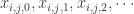$x_{i,j,0}, x_{i,j,1}, x_{i,j,2},\cdots$ of rational numbers converging to the left endpoint $L_{i,j}$ . Then let $A_{i,j,0}=[x_{i,j,0},R_{i,j}]$ , $A_{i,j,1}=[x_{i,j,1},x_{i,j,0}]$ , $A_{i,j,2}=[x_{i,j,2},x_{i,j,1}]$ , etc (see the following figure).

As in the previous step, two important points to consider in Step $2$ . One is that we make sure the rational number $r_2$ is chosen as an endpoint of some interval in Step 2. The second is that the length of each $A_{i,j,k}$ is less than $\displaystyle \frac{1}{2^2}$ .

___________________________________________________________________________
Remark

In the process described above, the endpoints of the intervals $A_{f(0),\cdots,f(n)}$ are rational numbers and we make sure that all the rational numbers are used as endpoints. We also make sure that the intervals from the successive steps are nested closed intervals with lengths $\rightarrow 0$ . The consequence of this point is that the nested decreasing closed intervals will collapse to one single point (since the real line is a complete metric space) and this single point must be an irrational number (since all the rational numbers are used up as endpoints of the nested closed intervals).

In Step $i$ where $i$ is an odd integer, we make the endpoints of the new intervals converge to the right. In Step $i$ where $i>1$ is an even integer, we make the endpoints of the new intervals converge to the left. This manipulation is to ensure that the nested closed intervals will never share the same endpoint from one step all the way to the end of the process.

Thus if we have $f \in \omega^\omega$ , then $\bigcap \limits_{n=0}^\infty A_{f(0),\cdots,f(n)} \ne \varnothing$ and in fact has only one point that is an irrational number.

On the other hand, for each point $x \in \mathbb{P}$ , we can locate inductively a sequence of intervals, $A_{f(0)}, A_{f(0),f(1)}, A_{f(0),f(1),f(2)}, \cdots$ , containing the point $x$ . This sequence of nested closed intervals must collapse to a single point and the single point must be the irrational number $x$ .

The process described above gives us a one-to-one mapping from $\mathbb{P}$ onto the product space $\omega^\omega$ . This mapping is also continuous in both directions, making it a homeomorphism. the nested intervals defined above form a base for the Euclidean topology on $\mathbb{P}$ . These basic open sets have a natural correspondance with basic open sets in the product space $\omega^\omega$ .

For example, for $f \in \omega^\omega$ , $\left\{ A_{f(0),\cdots,f(n)} \cap \mathbb{P}: n \in \omega \right\}$ is a local base at the point $x \in \bigcap \limits_{n=0}^\infty A_{f(0),\cdots,f(n)}$ . One the other hand, each $A_{f(0),\cdots,f(n)} \cap \mathbb{P}$ has a natural counterpart in a basic open set in the product space, namely the following set:

$\displaystyle . \ \ \ \ \left\{g \in \omega^\omega: g \restriction n = f \restriction n \right\}$

___________________________________________________________________________

The above process establishes that the countable product of the integers, $\omega^\omega$ , is equivalent topologically to the Euclidean space $\mathbb{P}$ .

When is a Lindelof Space Normal?

Posted on May 3, 2012 by Dan Ma

When is a Lindelof space normal? This question may seem strange since it is a well known basic result that Lindelof spaces are normal (see Theorem 3.8.2 in [1] and Theorem 16.8 in [6]). The proofs in both of these theorems require that the Lindelof space is also a regular space. We present an example showing that the requirement of regularity cannot be removed. The example defined below is a space that is Hausdorff, hereditarily Lindelof, not separable, not regular and not normal.

The example defined below makes it clear that we need to be careful in making the leap from the Lindelof property to normality of a space. We need to make sure that the space in question is also a regular space. The Lindelof property is a powerful property; it also implies paracompactness. But for this to happen, some separation axiom is required (it needs to be a regular space).

Another motivation for looking at examples such as the one defined here is that they are background information to the theory of S-spaces and L-spaces (see the remark given at the end of the post).

______________________________________________________________________________

The example is the Example 14.7 in [2]. The underlying set is the real number line $\mathbb{R}$ . Let $\tau$ be the usual topology on $\mathbb{R}$ . Let $X=\mathbb{R}$ . We use the following collection of sets as a base for a new topology on $X$ :

$\displaystyle \mathbb{B}=\left\{O-C: O \in \tau, C \subset \mathbb{R}, \lvert C \vert \le \omega \right\}$

The collection $\mathbb{B}$ needs to satisfy two conditions for being a base for a topology. One is that it covers the underlying set. The second is that whenever $B_1, B_2 \in \mathbb{B}$ with $x \in B_1 \cap B_2$ , there is some $B_3 \in \mathbb{B}$ such that $x \in B_3 \subset B_1 \cap B_2$ . Note that $\tau \subset \mathbb{B}$ . This implies that $\mathbb{B}$ is a cover of $X$ . It is also clear that the second condition is satisfied.

Let $\tau^{*}$ be the topology generated by the base $\mathbb{B}$ . Another consequence of $\tau \subset \mathbb{B}$ is that the new topology on $X$ is finer than the usual topology, i.e., $\tau \subset \tau^{*}$ . It is then clear that $(X, \tau^{*})$ is a Hausdorff space.

We denote the real line with the new topology $\tau^{*}$ by $X$ rather than $(X, \tau^{*})$ since the new topology $\tau^{*}$ is the primary focus.

In $X$ , the complement of every countable set is open. So no countable set can be dense in $X$ , making it not separable. Equivalently, every countable subset of $X$ is closed.

To see that $X$ is not regular, we first make the following observation.

Observation
Let $W \subset \mathbb{R}$ be a Euclidean open set. Let $A \subset \mathbb{R}$ be a countable set that is dense in $W$ (dense with respect to the Euclidean topology). Then for each $x \in A \cap W$ , $x \in \overline{W-A}$ (with respect to the topology $\tau^*$ ).

To see that this observation is correct, let $x \in A \cap W$ and let $V-B$ be an open set containing $x$ , where $V$ is a Euclidean open set and $B$ is a countable set. We can assume that $V \subset W$ . Let $A_0=A-\left\{x \right\}$ . Note that $x \in V-(A_0 \cup B) \subset V-B$ and that $V-(A_0 \cup B) \subset W-A_0$ . Furthermore, for any $y \in V-(A_0 \cup B)$ with $y \ne x$ , $y \in W-A$ . Thus any open set containing $x$ contains many points of $W-A$ . Hence, we have $x \in \overline{W-A}$ .

To see that $X$ is not regular, we show that there is a closed set $C \subset X$ such that for any open set $O \subset X-C$ , $\overline{O} \cap C \ne \varnothing$ .

Let $C=\mathbb{Q}$ (the set of all rational numbers). Let $O$ be open in $X$ such that $O \subset X-C$ . We assume that $O=W-A$ where $W$ is open in the Euclidean topology and $A$ is countable. Note that $O=W-A$ consisting of entirely of irrational numbers. Then $\mathbb{Q} \cap W \subset A$ . Thus $A$ is dense in $W$ (with respect to the Euclidean topology). By the above observation, any point of $A$ is a member of $\overline{W-A}$ (with respect to the topology $\tau^*$ ). In particular, for each $x \in C=\mathbb{Q}$ , $x \in \overline{W-A}$ . Thus $X$ is not regular.

Any space that is not regular is also not normal. Thus $X$ is not normal. But we can also see this directly. Let $H=\mathbb{Q}$ and $K=\left\{x \right\}$ where $x$ is any irrational number. Then $H$ and $K$ are two disjoint closed sets that cannot be separated by disjoint open sets in $X$ .

The space $X$ is Lindelof and also hereditarily Lindelof (both properties are piggy backed on the same properties of the Euclidean real line). To see that $X$ is Lindelof, suppose that a collection of open sets $O_a-A_a \in \mathbb{B}$ is a cover of $X$ . The Euclidean open sets $O_a$ also form a cover of $X=\mathbb{R}$ . Then pick countably many $O_a$ that also cover the real line (using the Lindelof property of the Euclidean real line). Then these countably many $O_a-A_a$ will cover $X$ except for countably many points. A countable subcover will result once we use open sets in the original cover to cover these countably many points. Using the same proof, it can be shown that every subspace of $X$ is also Lindelof.

______________________________________________________________________________

Remark

An S-space is any regular topological space that is hereditarily separable but not Lindelof. An L-space is any regular topological space that is hereditarily Lindelof but not separable. Elementary examples of hereditarily separable space that is not Lindelof and hereditarily Lindelof space that is not separable are quite easy to define (but they are not regular). The example we define above is an example of non-regular hereditarily Lindelof space that is not separable. Thus S-space and L-space are typically defined with the requirement of regularity.

It was shown in the early 1980’s that the existence of S-space is independent of the usual axioms of ZFC. This means that to prove the existence of an S-space or to prove the non-existence of S-space, one needs to assume axioms beyond those of ZFC. The L-space problem (whether an L-space can exist without assuming additional set-theoretic assumptions beyond those of ZFC) was not resolved until quite recently. For quite a long time, it was believed the L-space problem would have a similar solution (that its existence would be independent of ZFC). In 2005, Justin Tatch-Moore solved the L-space problem by constructing an L-space without assuming additional axioms.

For back ground information about S-space and L-space, see [3] and [4]. For Justin Moore’s proof, see [5].

______________________________________________________________________________

Reference

Engelking, R., General Topology, Revised and Completed edition, 1989, Heldermann Verlag, Berlin.
Hodel, R.,Cardinal Functions I, Handbook of Set-Theoretic Topology, (K. Kunen and J. E. Vaughan, eds), 1984, Elsevier Science Publishers B. V., Amsterdam, 1-61.
Mastros, S.,S and L Spaces, Master’s Thesis, 2009, University of Pittsburgh. Link
Roitman, J.,Basic S and L, Handbook of Set-Theoretic Topology, (K. Kunen and J. E. Vaughan, eds), 1984, Elsevier Science Publishers B. V., Amsterdam, 295-326.
Tatch-Moore, J.,A solution to the L space problem, Journal of the American Mathematical Society, 19 (2006), 3, 717—736. Link
Willard, S., General Topology, 1970, Addison-Wesley Publishing Company.

Elementary Examples of Lindelof Spaces and Separable Spaces

Posted on April 29, 2012 by Dan Ma

The Euclidean spaces $\mathbb{R}$ and $\mathbb{R}^n$ are both Lindelof and separable. In fact these two properties are equivalent in the class of metrizable spaces. A space is metrizable if its topology can be induced by a metric. In a metrizable space, having one of these properties implies the other one. Any students in beginning topology courses who study basic notions such as the Lindelof property and separability must venture outside the confine of Euclidean spaces or metric spaces. The goal of this post is to present some elementary examples showing that these two notions are not equivalent.

All topological spaces under consideration are Hausdorff. Let $X$ be a space. Let $D \subset X$ . The set $D$ is said to be dense in $X$ if every nonempty open subset of $X$ contains some point of $D$ . The space $X$ is said to be separable if there is countable subset of $X$ that is also dense in $X$ . All Euclidean spaces are separable. For example, in the real line $\mathbb{R}$ , every open interval contains a rational number. Thus the set of all rational numbers $\mathbb{Q}$ is dense in $\mathbb{R}$ .

Let $\mathcal{U}$ be a collection of subsets of the space $X$ . The collection $\mathcal{U}$ is said to be a cover of $X$ if every point of $X$ is contained in some element of $\mathcal{U}$ . The collection $\mathcal{U}$ is said to be an open cover of $X$ if, in addition it being a cover, $\mathcal{U}$ consists of open sets in $X$ .

Let $\mathcal{U}$ be a cover of the space $X$ . Let $\mathcal{V} \subset \mathcal{U}$ . If the collection $\mathcal{V}$ is also a cover of $X$ , we say that $\mathcal{V}$ is a subcover of $\mathcal{U}$ . The space $X$ is a Lindelof space (or has the Lindelof property) if every open cover of $X$ has a countable subcover.

The real $\mathbb{R}$ is Lindelof. Both the Lindelof property and the separability of $\mathbb{R}$ follows from the fact that the Euclidean topology on $\mathbb{R}$ can be generated by a countable base (e.g. one countable base consists of all open intervals with rational endpoints). Now some non-Euclidean (and non-metrizable) examples.

__________________________________________________________________________________

Example 1 – A Lindelof space that is not separable
Let $X$ be any uncountable set. Let $p$ be a point that is not in $X$ , e.g., let $p=\left\{ X \right\}$ . Define the space $Y = \left\{p\right\} \cup X$ as follows. Let every point in $X$ be isolated, meaning any singleton set $\left\{ x \right\}$ is declared open for any $x \in X$ . An open neighborhood of the point $p$ is of the form $\left\{p\right\} \cup W$ where $X-W$ is a countable subset of $X$ .

It is clear that the resulting space $Y$ is Lindelof since every open set containing $p$ contains all but countably many points of $X$ . It is also clear that no countable set can be dense in $Y$ .

Even though this example $Y$ is Lindelof, it is not hereditarily Lindelof since the subspace $X$ is uncountable discrete space.

In a previous post, we showed that the space $Y$ defined in this example is a productively Lindelof space (meaning that its product with every Lindelof space is Lindelof).

__________________________________________________________________________________
Remark

A space is said to have the countable chain condition (CCC) if there are no uncountable family of pairwise disjoint open subsets. It is clear that any separable space has the CCC. It follows that the space $Y$ in Example 1 does not have the CCC, since the singleton sets $\left\{ x \right\}$ (with $x \in X$ ) forms a pairwise disjoint collection of open sets, showing that the Lindelof property does not even imply the weaker property of having the CCC.

__________________________________________________________________________________

Example 2 – A separable space that is not Lindelof
The example here is the Tangent Disc Space (Niemytzki’s Tangent Disc Topology in [2]). The underlying set is the upper half plane (the x-axis and the plane above the x-axis). In other words, consider the following set:

$\displaystyle . \ \ \ \ \ X=\left\{(x,y) \in \mathbb{R}^2: y \ge 0 \right\}$

Let $\displaystyle X_u=\left\{(x,y) \in \mathbb{R}^2: y>0 \right\}$ and $T=\left\{(x,0): x \in \mathbb{R} \right\}$ . The line $T$ is the x-axis and $X_u$ is the upper plane without the x-axis. We define a topology on $X$ such that $X_u$ as a subspace in this topology is Euclidean. The open neighborhoods of a point $p=(x,0) \in T$ are of the form $\left\{p \right\} \cup D$ where $D$ is an open disc tangent to the x-axis at the point $p$ . The figure below illustrates how open neighborhoods at the x-axis are defined.

It is clear that the points with rational coordinates in the upper half plane $X_u$ form a dense set in the tangent disc topology. Thus $X$ is separable. In any Lindelof space, there are no uncountable closed and discrete subsets. Note that the x-axis $T$ is a closed and discrete subspace in the tangent disc space. Thus $X$ is not Lindelof.

Though separable, the Tangent Disc Space is not hereditarily separable since the x-axis $T$ is uncountable and discrete.

The Tangent Disc Space is an interesting example. For example, it is a completely regular space that is an example of a Moore space that is not normal. For these and other interesting facts about the Tangent Disc Space, see [2].

__________________________________________________________________________________

For the Lindelof property and the property of being separable, there are plenty of examples of spaces that possess only one of the properties. All three references indicated below are excellent places to look. The book by Steen and Seebach ([2]) is an excellent catalog of interesting spaces (many of them are elementary).
__________________________________________________________________________________

Reference

Engelking, R., General Topology, Revised and Completed edition, 1989, Heldermann Verlag, Berlin.
Steen, L. A., Seebach, J. A.,Counterexamples in Topology, 1995, Dover Edition, Dover Publications, New York.
Willard, S., General Topology, 1970, Addison-Wesley Publishing Company.

Sequential spaces, III

Posted on July 1, 2010 by Dan Ma

This is a continuation of the discussion on sequential spaces started with the post Sequential spaces, I and Sequential spaces, II and k-spaces, I. The topology in a sequential space is generated by the convergent sequences. The convergence we are interested in is from a topological view point and not necessarily from a metric (i.e. distance) standpoint. In our discussion, a sequence $\left\{x_n\right\}_{n=1}^\infty$ converges to $x$ simply means for each open set $O$ containing $x$ , $O$ contains $x_n$ for all but finitely many $n$ . In any topological space, there are always trivial convergent sequences. These are sequences of points that are eventually constant, i.e. the sequences $\left\{x_n\right\}$ where for some $n$ , $x_n=x_j$ for $j \ge n$ . Any convergent sequence that is not eventually constant is called a non-trivial convergent sequence. We present an example of a space where there are no non-trivial convergent sequences of points. This space is derived from the Euclidean topology on the real line. This space has no isolated point in this space and yet has no non-trivial convergent sequences and has no infinite compact sets. From this example, we make some observations about sequential spaces and k-spaces.

The space we define here is obtained by modifying the Euclidean topology on the real line. Let $\mathbb{R}$ be the real line. Let $\tau_e$ be the Euclidean topology on the real line. Consider the following collection of subsets of the real line:

$\mathcal{B}=\left\{U-C:U \in \tau_e \text{ and } \lvert C \lvert \le \omega\right\}$

It can be verified that $\mathcal{B}$ is a base for a topology $\tau$ on $\mathbb{R}$ . In fact this topology is finer than the Euclidean topology. Denote $\mathbb{R}$ with this finer topology by $X$ . Clearly $X$ is Hausdorff since the Euclidean topology is. Any countable subset of $X$ is closed. Thus $X$ is not separable (no countable set can be dense). This space is a handy example of a hereditarily Lindelof space that is not separable. The following lists some properties of $X$ :

$X$ is herditarily Lindelof.
There are no non-trivial convergent sequences in $X$ .
All compact subsets of $X$ are finite.
$X$ is not a k-space and is thus not sequential.

Discussion of 1. This follows from the fact that the real line with the Euclidean topology is hereditarily Lindelof and the fact that each open set in $X$ is an Euclidean open set minus a countable set.

Discussion of 2 This follows from the fact that every countable subset of $X$ is closed. If a non-trivial sequence $\left\{x_n\right\}$ were to converge to $x \in X$ , then $\left\{x_n:n=1,2,3,\cdots\right\}$ would be a countable subset of $X$ that is not closed.

Discussion of 3. Let $A \subset X$ be an infinite set. If $A$ is bounded in the Euclidean topology, then there would be a non-trivial convergent sequence of points of $A$ in the Euclidean topology, say, $x_n \mapsto x$ . Let $U_0=X-\left\{x_n:n=1,2,3,\cdots\right\}$ , which is open in $X$ . For $n \ge 1$ , let $U_n$ be Euclidean open such that $x_n \in U_n$ . We also require that all $U_n$ are pairwise disjoint and not contain $x$ . Then $U_0,U_1,U_2,\cdots$ form an open cover of $A$ (in the topology of $X$ ) that has no finite subcover. So any bounded infinite $A$ is not compact in $X$ .

Suppose $A$ is unbounded in the Euclidean topology. Then $A$ contains a closed and discrete subset $\left\{x_1,x_2,x_3,\cdots\right\}$ in the Euclidean topology. We can find Euclidean open sets $U_n$ that are pairwise disjoint such that $x_n \in U_n$ for each $n$ . Let $U_0=X-\left\{x_n:n=1,2,3,\cdots\right\}$ , which is open in $X$ . Then $U_0,U_1,U_2,\cdots$ form an open cover of $A$ (in the topology of $X$ ) that has no finite subcover. So any unbounded infinite $A$ is not compact in $X$ .

Discussion of 4. Note that every point of $X$ is a non-isolated point. Just pick any $x \in X$ . Then $X-\left\{x\right\}$ is not closed in $X$ . However, according to 3, $K \cap (X-\left\{x\right\})$ is finite and is thus closed in $K$ for every compact $K \subset X$ . Thus $X$ is not a k-space.

General Discussion
Suppose $\tau$ is the topology for the space $Y$ . Let $\tau_s$ be the set of all sequentially open sets with respect to $\tau$ (see Sequential spaces, II). Let $\tau_k$ be the set of all compactly generated open sets with respect to $\tau$ (see k-spaces, I). The space $Y$ is a sequential space (a k-space ) if $\tau=\tau_s$ ( $\tau=\tau_k$ ). Both $\tau_s$ and $\tau_k$ are finer than $\tau$ , i.e. $\tau \subset \tau_s$ and $\tau \subset \tau_k$ . When are $\tau_s$ and $\tau_k$ discrete? We discuss sequential spaces and k-spaces separately.

Observations on Sequential Spaces
With respect to the space $(Y,\tau)$ , we discuss the following four properties:

A. $\$ No non-trivial convergent sequences.
B. $\$ $\tau_s$ is a discrete topology.
C. $\$ $\tau$ is a discrete topology.
D. $\$ Sequential, i.e., $\tau=\tau_s$ .

Observation 1
The topology $\tau_s$ is discrete if and only if $Y$ has no non-trivial convergent sequences, i.e. $A \Longleftrightarrow B$ .

If $\tau_s$ is a discrete topology, then every subset of $Y$ is sequentially open and every subset is sequentially closed. Hence there can be no non-trivial convergent sequences. If there are no non-trivial convergent sequences, every subset of the space is sequentially closed (thus every subset is sequentially open).

Observation 2
Given that $Y$ has no non-trivial convergent sequences, $Y$ is not discrete if and only if $Y$ is not sequential. Equivalently, given property A, $C \Longleftrightarrow D$ .

Given that there are no non-trivial convergent sequences in $Y$ , $\tau_s$ is discrete. For $(Y,\tau)$ to be sequential, $\tau=\tau_s$ . Thus for a space $Y$ that has no non-trivial convergent sequences, the only way for $Y$ to be sequential is that it is a discrete space.

Observation 3
Given $Y$ is not discrete, $Y$ has no non-trivial convergent sequences implies that $Y$ is not sequential, i.e. given $\text{not }C$ , $A \Longrightarrow \text{not }D$ . The converse does not hold.

Observation 3 is a rewording of observation 2. To see that the converse of observation 3 does not hold, consider $Y=[0,\omega_1]=\omega_1+1$ , the successor ordinal to the first uncountable ordinal with the order topology. It is not sequential as the singleton set $\left\{\omega_1\right\}$ is sequentially open and not open.

Observations on k-spaces
The discussion on k-spaces mirrors the one on sequential spaces. With respect to the space $(Y,\tau)$ , we discuss the following four properties:

E. $\$ No infinite compact sets.
F. $\$ $\tau_k$ is a discrete topology.
G. $\$ $\tau$ is a discrete topology.
H. $\$ k-space, i.e., $\tau=\tau_k$ .

Observation 4
The topology $\tau_k$ is discrete if and only if $Y$ has no infinite compact sets, i.e. $E \Longleftrightarrow F$ .

If $\tau_k$ is a discrete topology, then every subset of $Y$ is a compactly generated open set. In particular, for every compact $K \subset Y$ , every subset of $K$ is open in $K$ . This means $K$ is discrete and thus must be finite. Hence there can be no infinite compact sets if $\tau_k$ is discrete. If there are no infinite compact sets, every subset of the space is a compactly generated closed set (thus every subset is a compactly generated open set).

Observation 5
Given that $Y$ has no infinite compact sets, $Y$ is not discrete if and only if $Y$ is not a k-space. Equivalently, given property E, $G \Longleftrightarrow H$ .

Given that there are no infinite compact sets in $Y$ , $\tau_k$ is discrete. For $(Y,\tau)$ to be a k-space, $\tau=\tau_k$ . Thus for a space $Y$ that has no infinite compact sets, the only way for $Y$ to be a k-space is that it is a discrete space.

Observation 6
Given $Y$ is not discrete, $Y$ has no infinite compact sets implies that $Y$ is not a k-space, i.e. given $\text{not }G$ , $E \Longrightarrow \text{not }H$ . The converse does not hold.

Observation 6 is a rewording of observation 5. To see that the converse of observation 6 does not hold, consider the topological sum of a non-k-space and an infinite compact space.

Remark
In the space $X$ defined above by removing countable sets from Euclidean open subsets of the real line, there are no infinite compact sets and no non-trivial convergent sequences. Yet the space is not discrete. Thus it can neither be a sequential space nor a k-space. Another observation we would like to make is that no infinite compact sets implies no non-trivial convergent sequences ( $E \Longrightarrow A$ ). However, the converse is not true. Consider $\beta(\omega)$ , the Stone-Cech compactification of $\omega$ , the set of all nonnegative integers.

Reference

Engelking, R. General Topology, Revised and Completed edition, 1989, Heldermann Verlag, Berlin.
Willard, S., General Topology, 1970, Addison-Wesley Publishing Company.

Perfect sets and Cantor sets, II

Posted on May 30, 2010 by Dan Ma

This is post #11 of the series on the Euclidean topology of the real line. See the links at the bottom for other posts in the series.

In the previous post Perfect sets and Cantor sets, I, we show that every nonempty perfect set is uncountable. We now show that any perfect contains a Cantor set. Hence the cardinality of any perfect set is continuum.

Given a perfect set $W$ , we construct a Cantor set within $W$ . Consider the following cases:

Case 1. $W$ contains some bounded closed interval $[a,b]$ .
Case 2. $W$ does not any bounded closed interval.

If case 1 holds, then we can apply the middle third process on $[a,b]$ and produce a Cantor set. So in the remaining dicussion of this post, we assume case 2 holds. This means that for each closed interval $[a,b]$ , there is some $x \in [a,b]$ such that $x \notin W$ .

Background Discussion
Let $A \subset \mathbb{R}$ and $p \in A$ . The point $p$ is a right-sided limit point of $A$ if for each open interval $(a,b)$ containing $p$ , the open interval $(p,b)$ contains a point of $A$ . The point $p$ is a left-sided limit point of $A$ if for each open interval $(a,b)$ containing $p$ , the open interval $(a,p)$ contains a point of $A$ . The point $p$ is a two-sided limit point of $A$ if it is both a right-sided limit point and a left-sided limit point of $A$ . For the proof of the following lemma, see the post labeled #10 listed below.

In Lemma 2 below, we apply the least upper bound property and the greatest lower bound property. See the post labeled #4 listed below.

Key Lemmas for Construction

Lemma 1
Suppose that $X \subset \mathbb{R}$ is an uncountable set. Then $X$ contains a two-sided limit point.

As a corollary to the lemma 1, for the perfect set $W$ in question, all but countably many points of $W$ are two-sided limit points of $W$ .

Lemma 2
Suppose $E \subset \mathbb{R}$ is a nonempty perfect set that satisfies Case 2 indicated above. Suppose that for the closed interval $[a,b]$ , we have:

$(a,b) \cap E \ne \phi$ ,
the left endpoint $a$ is a right-sided limit point of $E$ ,
the right endpoint $b$ is a left-sided limit point of $E$ .

Then we have $a<a^*<b^*<b$ such that:

there are no points of $E$ in the open interval $(a^*,b^*)$ ,
the point $a^*$ is a left-sided limit point of $E$ ,
the point $b^*$ is a right-sided limit point of $E$ .

Proof. Since Case 2 holds, for the closed interval $[a,b]$ in question, there is some $x \in (a,b)$ such that $x \notin E$ . Then we can find an open interval $(c,d)$ such that $x \in (c,d)$ and $a<c<d<b$ and $(c,d) \cap E = \phi$ .

Any point in $(c,d)$ is an upper bound of $W_1=[a,c) \cap E$ . By the least upper bound property, $W_1$ has a least upper bound $a^*$ . Any point in $(c,d)$ is an lower bound of $W_2=(d,b] \cap E$ . By the greatest lower bound property, $W_2$ has a greatest lower bound $b^*$ . Then $a^*$ and $b^*$ satisfy the conclusion of the lemma. $\blacksquare$

Lemma 3
Suppose $E \subset \mathbb{R}$ is a nonempty perfect set. Suppose we have a closed interval $[s,t]$ such that the left endpoint $s$ is a right-sided limit point of $E$ and the right endpoint $t$ is a left-sided limit points of $E$ . Then we have $s<s_*<t_*<t$ such that:

the open interval $(s_*,t_*)$ contains points of $E$ ,
both endpoints $s_*$ and $t_*$ are two-sided limit points of $E$ ,
$t_*-s_*<0.5(t-s)$ .

Proof. Suppose we have a closed interval $[s,t]$ as described in the lemma. Then $E_1=[s,t] \cap E$ is a nonempty perfect set. Thus $E_1$ is uncountable. So pick $p \in (s,t)$ such that $p$ is a two-sided limit point of $E_1$ .

Choose open interval $(c,d)$ such that $s<c<p<d<t$ and $d-c<0.5(t-s)$ . Since $p$ is a two-sided limit point of $E_1$ , choose $s^*$ and $t^*$ such that $c<s^*<p$ , $p<t^*<d$ and both $s^*$ and $t^*$ are two-sided limit points of $E_1$ . It follows that $s^*$ and $t^*$ satisfy the conclusion of the lemma. $\blacksquare$

Lemma 4
Suppose $E \subset \mathbb{R}$ is a nonempty perfect set that satisfies Case 2 indicated above. Suppose we have a closed interval $[a,b]$ such that the endpoints are two-sided limit points of $E$ . Then we have disjoint closed intervals $K_0=[p_0,q_0]$ and $K_1=[p_1,q_1]$ such that

$K_0 \subset [a,b]$ and $K_1 \subset [a,b]$ ,
the lengths of both $K_0$ and $K_1$ are less then $0.5(b-a)$ ,
for each of $K_0$ and $K_1$ , the endpoints are two-sided limit points of $E$ .

Proof. This is the crux of the construction of a Cantor set from a perfect set and is the result of applying Lemma 2 and Lemma 3.

Applying Lemma 2 on $[a,b]$ and obtain the open interval $(a^*,b^*)$ . We remove the open interval $(a^*,b^*)$ from $[a,b]$ and obtain two disjoint closed intervals $[a,a^*]$ and $[b^*,b]$ . Each of these two subintervals contains points of the perfect set $W$ since the endpoints are limit points of $W$ in the correct direction.

Now apply Lemm 3 to shrink $[a,a^*]$ to obtain a smaller subinterval $K_0=[p_0,q_0]$ such that the length of $K_0$ is less than $0.5(a^*-a)$ and is thus less than $0.5(b-a)$ . Likewise, apply Lemma 3 on $[b^*,b]$ to obtain $K_1=[p_1,q_1]$ such that the length of $K_1$ is less than $0.5(b-b^*)$ and is thus less than $0.5(b-a)$ . Note that both $K_0$ and $K_1$ constain points of $E$ , making both $K_0 \cap E$ and $K_1 \cap E$ perfect sets and compact sets. $\blacksquare$

Construction
Suppose $W \subset \mathbb{R}$ is a nonempty perfect set that satisfies Case 2. Pick two two-sided limit $a_0$ and $b_0$ of $W$ . Obtain $B_0=K_0$ and $B_1=K_1$ as a result of applying Lemma 4. Let $A_1=B_0 \cup B_1$ .

Then we apply Lemma 4 on the closed interval $B_0$ and obtain closed intervals $B_{00}$ , $B_{01}$ . Likewise we apply Lemma 4 on the closed interval $B_1$ and obtain closed intervals $B_{10}$ , $B_{11}$ . Let $A_2=B_{00} \cup B_{01} \cup B_{10} \cup B_{11}$ .

Continue this induction process. Let $C=\bigcap \limits_{n=1}^{\infty} A_n$ . The set $C$ is a Cantor set and has all the properties discussed in the posts labled #6 and #7 lised at the end of this post.

We claim that $C \subset W$ . For any countably infinite sequence $g$ of zeros and ones, let $g_n$ be the first $n$ terms in $g$ . Let $y \in C$ . Then $\left\{y\right\}=\bigcap \limits_{n=1}^{\infty} B_{g_n}$ for some countably infinite sequence $g$ of zeros and ones (see post #6 listed below). Then every open interval $(a,b)$ containing $y$ would contain some closed interval $B_{g_n}$ . Thus $y$ is a limit point of $W$ . Hence $y \in W$ .

Links to previous posts on the topology of the real line:
1. The Euclidean topology of the real line (1)
2. The Euclidean topology of the real line (2)
3. The Euclidean topology of the real line (3) – Completeness
4. The Euclidean topology of the real line (4) – Compactness
5. The Cantor bus tour
6. The Cantor set, I
7. The Cantor set, II
8. The Cantor set, III
9. Perfect sets and Cantor sets, I
10. The Lindelof property of the real line

Perfect sets and Cantor sets, I

Posted on May 27, 2010 by Dan Ma

This is post #9 of the series on the Euclidean topology of the real line. See the links at the bottom for other posts in the series.

Recall that a subset $A$ of the real line is a perfect set if $A$ is closed in Euclidean topology of the real line and that every point of $A$ is a limit point of $A$ . Any closed and bounded interval $[a,b]$ is a perfect set. The Cantor sets (the middle third version and other variations) are perfect sets (see the links #7 and #8 below). It turns out that any nonempty perfect set contains a Cantor set. In this series of posts on Euclidean topology of the real line, by Cantor sets we mean any set that can be constructed by a binary process of splitting closed intervals into two halves at each stage (see links for #6 and #8 below). We demonstrate the algorithm of constructing a Cantor set from any perfect set. This post (part I) shows that any nonempty perfect set is uncountable. Knowing that a perfect is uncountable will simplify the construction process (next post).

Suppose $W \subset \mathbb{R}$ is a nonempty perfect subset. We show that $W$ is uncountable. Since $W$ has at least one point and every point is a limit point, $W$ is infinite. The key to showing $W$ is uncountable is that every nested decreasing sequence of compact subsets of the real line (actually in any topological space) has nonempty intersection. If $W$ happens to be countable, we can define a nested sequence of compact subsets of $W$ with empty intersection. Thus $W$ cannot be countable.

The following lemma is a corollary to Theorem 3 in the post # 4 listed below. The lemma applies to any abstract spaces where compactness can be defined. We state the lemma in terms of the real line since this is our focus.

Lemma
Suppose $C_1,C_2,C_3, \cdots$ are compact subsets of the real line such that

$\displaystyle C_1 \supset C_2 \supset C_3 \supset \cdots$ .

Then $\bigcap \limits_{n=1}^{\infty} C_n \ne \phi$ .

To make the argument that $W$ is uncountable more precise, suppose that $W$ is countable. Then we can enumerate $W$ in a sequence indexed by the positive integers. We have:

$\displaystyle W=\left\{w_1,w_2,w_3,\cdots\right\}$

Pick a bounded open interval $O_1$ such that $w_1 \in O_1$ . Next, pick an open interval $O_2$ such that $\overline{O_2} \subset O_1$ and $w_2 \notin \overline{O_2}$ and $O_2 \cap W \ne \phi$ .

In the $n^{th}$ stage where $n \ge 2$ , pick an open interval $O_n$ such that $\overline{O_n} \subset O_{n-1}$ and $w_n \notin \overline{O_n}$ and $O_n \cap W \ne \phi$ . Since $W$ is a perfect set, the induction step can continue at every stage.

Now, let $C_n=\overline{O_n} \cap W$ . Note that $C_n$ is a compact set since $\overline{O_n}$ is compact. By the lemma, the intersection of the $C_n$ must be nonempty. By the induction steps, no point of $W$ belongs to all the sets $\overline{O_n}$ , implying the intersection of $C_n$ is empty, a contradiction. Thus $W$ must be uncountable.

Remark
As a corollary, the real line and the unit intervals are uncountable. A more interesting corollary is that any nonempty perfect set has a two-sided limit point. In fact all but countably many points of a nonempty perfect set are two sided limit points. See the post The Lindelof property of the real line for a proof that any uncountable subset of the real line has a two sided limit point. This fact will simplify the construction of a Cantor set from a perfect set.

Reference

Rudin, W., Principles of Mathematical Analysis, Third Edition, 1976, McGraw-Hill, Inc, New York.

Dan Ma's Topology Blog

Expository Articles In General Topology

Tag Archives: Euclidean topology

Bernstein Sets Are Baire Spaces

A Question About The Rational Numbers

Thinking about the Space of Irrationals Topologically

When is a Lindelof Space Normal?

Elementary Examples of Lindelof Spaces and Separable Spaces

Sequential spaces, III

Perfect sets and Cantor sets, II

Perfect sets and Cantor sets, I