In this post, we introduce a class of hyperspaces called Pixley-Roy spaces. This is a well-known and well studied set of topological spaces. Our goal here is not to be comprehensive but rather to present some selected basic results to give a sense of what Pixley-Roy spaces are like.
A hyperspace refers to a space in which the points are subsets of a given “ground” space. There are more than one way to define a hyperspace. Pixley-Roy spaces were first described by Carl Pixley and Prabir Roy in 1969 (see [5]). In such a space, the points are the non-empty finite subsets of a given ground space. More precisely, let  be a
be a  space (i.e. finite sets are closed). Let
 ![\mathcal{F}[X]](https://s0.wp.com/latex.php?latex=%5Cmathcal%7BF%7D%5BX%5D&bg=ffffff&fg=333333&s=0&c=20201002) be the set of all non-empty finite subsets of . For each
be the set of all non-empty finite subsets of . For each ![F \in \mathcal{F}[X]](https://s0.wp.com/latex.php?latex=F+%5Cin+%5Cmathcal%7BF%7D%5BX%5D&bg=ffffff&fg=333333&s=0&c=20201002) and for each open subset
and for each open subset  of with
  , we define:
The sets ![[F,U]](https://s0.wp.com/latex.php?latex=%5BF%2CU%5D&bg=ffffff&fg=333333&s=0&c=20201002) over all possible
over all possible  and form a base for a topology on . This topology is called the Pixley-Roy topology (or Pixley-Roy hyperspace topology). The set with this topology is called a Pixley-Roy space.
The hyperspace as defined above was first defined by Pixley and Roy on the real line (see [5]) and was later generalized by van Douwen (see [7]). These spaces are easy to define and is useful for constructing various kinds of counterexamples. Pixley-Roy played an important part in answering the normal Moore space conjecture. Pixley-Roy spaces have also been studied in their own right. Over the years, many authors have investigated when the Pixley-Roy spaces are metrizable, normal, collectionwise Hausdorff, CCC and homogeneous. For a small sample of such investigations, see the references listed at the end of the post. Our goal here is not to discuss the results in these references. Instead, we discuss some basic properties of Pixley-Roy to solidify the definition as well as to give a sense of what these spaces are like. Good survey articles of Pixley-Roy are [3] and [7].
____________________________________________________________________
Basic Discussion
In this section, we focus on properties that are always possessed by a Pixley-Roy space given that the ground space is at least . Let be a space. We discuss the following points:
- The topology defined above is a legitimate one, i.e., the sets indeed form a base for a topology on .
- is a Hausdorff space.
- is a zero-dimensional space.
- is a completely regular space.
- is a hereditarily metacompact space.
Let ![\mathcal{B}=\left\{[F,U]: F \in \mathcal{F}[X] \text{ and } U \text{ is open in } X \right\}](https://s0.wp.com/latex.php?latex=%5Cmathcal%7BB%7D%3D%5Cleft%5C%7B%5BF%2CU%5D%3A+F+%5Cin+%5Cmathcal%7BF%7D%5BX%5D+%5Ctext%7B+and+%7D+U+%5Ctext%7B+is+open+in+%7D+X+%5Cright%5C%7D&bg=ffffff&fg=333333&s=0&c=20201002) . Note that every finite set belongs to at least one set in
. Note that every finite set belongs to at least one set in  , namely
 ![[F,X]](https://s0.wp.com/latex.php?latex=%5BF%2CX%5D&bg=ffffff&fg=333333&s=0&c=20201002) . So is a cover of . For
. So is a cover of . For ![A \in [F_1,U_1] \cap [F_2,U_2]](https://s0.wp.com/latex.php?latex=A+%5Cin+%5BF_1%2CU_1%5D+%5Ccap+%5BF_2%2CU_2%5D&bg=ffffff&fg=333333&s=0&c=20201002) , we have
, we have ![A \in [A,U_1 \cap U_2] \subset [F_1,U_1] \cap [F_2,U_2]](https://s0.wp.com/latex.php?latex=A+%5Cin+%5BA%2CU_1+%5Ccap+U_2%5D+%5Csubset+++%5BF_1%2CU_1%5D+%5Ccap+%5BF_2%2CU_2%5D&bg=ffffff&fg=333333&s=0&c=20201002) . So is indeed a base for a topology on .
. So is indeed a base for a topology on .
To show is Hausdorff, let  and
and  be finite subsets of where
  . Then one of the two sets has a point that is not in the other one. Assume we have
  . Since is , we can find open sets
  such that
  ,
,  and
and  . Then
 ![[A,U \cup V]](https://s0.wp.com/latex.php?latex=%5BA%2CU+%5Ccup+V%5D&bg=ffffff&fg=333333&s=0&c=20201002) and
and ![[B,V]](https://s0.wp.com/latex.php?latex=%5BB%2CV%5D&bg=ffffff&fg=333333&s=0&c=20201002) are disjoint open sets containing and respectively.
are disjoint open sets containing and respectively.
To see that is a zero-dimensional space, we show that is a base consisting of closed and open sets. To see that is closed, let ![C \notin [F,U]](https://s0.wp.com/latex.php?latex=C+%5Cnotin+%5BF%2CU%5D&bg=ffffff&fg=333333&s=0&c=20201002) . Either
. Either  or
or  . In either case, we can choose open
  with
with  such that
 ![[C,V] \cap [F,U]=\varnothing](https://s0.wp.com/latex.php?latex=%5BC%2CV%5D+%5Ccap+%5BF%2CU%5D%3D%5Cvarnothing&bg=ffffff&fg=333333&s=0&c=20201002) .
.
The fact that is completely regular follows from the fact that it is zero-dimensional.
To show that is metacompact, let  be an open cover of . For each , choose
  such that
  and let
 ![V_F=[F,X] \cap G_F](https://s0.wp.com/latex.php?latex=V_F%3D%5BF%2CX%5D+%5Ccap+G_F&bg=ffffff&fg=333333&s=0&c=20201002) . Then
. Then ![\mathcal{V}=\left\{V_F: F \in \mathcal{F}[X] \right\}](https://s0.wp.com/latex.php?latex=%5Cmathcal%7BV%7D%3D%5Cleft%5C%7BV_F%3A+F+%5Cin+%5Cmathcal%7BF%7D%5BX%5D+%5Cright%5C%7D&bg=ffffff&fg=333333&s=0&c=20201002) is a point-finite open refinement of . For each
is a point-finite open refinement of . For each ![A \in \mathcal{F}[X]](https://s0.wp.com/latex.php?latex=A+%5Cin+%5Cmathcal%7BF%7D%5BX%5D&bg=ffffff&fg=333333&s=0&c=20201002) , can only possibly belong to
, can only possibly belong to  for the finitely many
  .
.
A similar argument show that is hereditarily metacompact. Let ![Y \subset \mathcal{F}[X]](https://s0.wp.com/latex.php?latex=Y+%5Csubset+%5Cmathcal%7BF%7D%5BX%5D&bg=ffffff&fg=333333&s=0&c=20201002) . Let
. Let  be an open cover of
  . For each
  , choose
  such that
  and let
 ![W_F=([F,X] \cap Y) \cap H_F](https://s0.wp.com/latex.php?latex=W_F%3D%28%5BF%2CX%5D+%5Ccap+Y%29+%5Ccap+H_F&bg=ffffff&fg=333333&s=0&c=20201002) . Then
. Then  is a point-finite open refinement of . For each
  , can only possibly belong to
  for the finitely many such that .
____________________________________________________________________
More Basic Results
We now discuss various basic topological properties of . We first note that is a discrete space if and only if the ground space is discrete. Though we do not need to make this explicit, it makes sense to focus on non-discrete spaces when we look at topological properties of . We discuss the following points:
- If is uncountable, then is not separable.
- If is uncountable, then every uncountable subspace of is not separable.
- If is Lindelof, then is countable.
- If is Baire space, then is discrete.
- If has the CCC, then has the CCC.
- If has the CCC, then has no uncountable discrete subspaces,i.e., has countable spread, which of course implies CCC.
- If has the CCC, then is hereditarily Lindelof.
- If has the CCC, then is hereditarily separable.
- If has a countable network, then has the CCC.
- The Pixley-Roy space of the Sorgenfrey line does not have the CCC.
- If is a first countable space, then is a Moore space.
Bullet points 6 to 9 refer to properties that are never possessed by Pixley-Roy spaces except in trivial cases. Bullet points 6 to 8 indicate that can never be separable and Lindelof as long as the ground space is uncountable. Note that is discrete if and only if is discrete. Bullet point 9 indicates that any non-discrete can never be a Baire space. Bullet points 10 to 13 give some necessary conditions for to be CCC. Bullet 14 gives a sufficient condition for to have the CCC. Bullet 15 indicates that the hereditary separability and the hereditary Lindelof property are not sufficient conditions for the CCC of Pixley-Roy space (though they are necessary conditions). Bullet 16 indicates that the first countability of the ground space is a strong condition, making a Moore space.
__________________________________
To see bullet point 6, let be an uncountable space. Let  be any countable subset of . Choose a point
  that is not in any
  . Then none of the sets
  belongs to the basic open set
 ![[\left\{x \right\} ,X]](https://s0.wp.com/latex.php?latex=%5B%5Cleft%5C%7Bx+%5Cright%5C%7D+%2CX%5D&bg=ffffff&fg=333333&s=0&c=20201002) . Thus can never be separable if is uncountable.
. Thus can never be separable if is uncountable.
__________________________________
To see bullet point 7, let be uncountable. Let  . Let be any countable subset of . We can choose a point
  that is not in any . Choose some such that
  . Then none of the sets belongs to the open set
 ![[A ,X] \cap Y](https://s0.wp.com/latex.php?latex=%5BA+%2CX%5D+%5Ccap+Y&bg=ffffff&fg=333333&s=0&c=20201002) . So not only is not separable, no uncountable subset of is separable if is uncountable.
. So not only is not separable, no uncountable subset of is separable if is uncountable.
__________________________________
To see bullet point 8, note that has no countable open cover consisting of basic open sets, assuming that is uncountable. Consider the open collection ![\left\{[F_1,U_1],[F_2,U_2],[F_3,U_3],\cdots \right\}](https://s0.wp.com/latex.php?latex=%5Cleft%5C%7B%5BF_1%2CU_1%5D%2C%5BF_2%2CU_2%5D%2C%5BF_3%2CU_3%5D%2C%5Ccdots+%5Cright%5C%7D&bg=ffffff&fg=333333&s=0&c=20201002) . Choose that is not in any of the sets . Then
. Choose that is not in any of the sets . Then  cannot belong to
 ![[F_n,U_n]](https://s0.wp.com/latex.php?latex=%5BF_n%2CU_n%5D&bg=ffffff&fg=333333&s=0&c=20201002) for any
for any  . Thus can never be Lindelof if is uncountable.
__________________________________
For an elementary discussion on Baire spaces, see this previous post.
To see bullet point 9, let be a non-discrete space. To show is not Baire, we produce an open subset that is of first category (i.e. the union of countably many closed nowhere dense sets). Let a limit point (i.e. an non-isolated point). We claim that the basic open set ![V=[\left\{ x \right\},X]](https://s0.wp.com/latex.php?latex=V%3D%5B%5Cleft%5C%7B+x+%5Cright%5C%7D%2CX%5D&bg=ffffff&fg=333333&s=0&c=20201002) is a desired open set. Note that
is a desired open set. Note that  where
where
We show that each  is closed and nowhere dense in the open subspace
  . To see that it is closed, let
  with . We have
  . Then
 ![[A,X]](https://s0.wp.com/latex.php?latex=%5BA%2CX%5D&bg=ffffff&fg=333333&s=0&c=20201002) is open and every point of has more than points of the space . To see that is nowhere dense in , let
is open and every point of has more than points of the space . To see that is nowhere dense in , let ![[B,U]](https://s0.wp.com/latex.php?latex=%5BB%2CU%5D&bg=ffffff&fg=333333&s=0&c=20201002) be open with
be open with ![[B,U] \subset V](https://s0.wp.com/latex.php?latex=%5BB%2CU%5D+%5Csubset+V&bg=ffffff&fg=333333&s=0&c=20201002) . It is clear that
. It is clear that  where is open in the ground space . Since the point
  is not an isolated point in the space , contains infinitely many points of . So choose an finite set
  with at least
  points such that
  . For the the open set
 ![[C,U]](https://s0.wp.com/latex.php?latex=%5BC%2CU%5D&bg=ffffff&fg=333333&s=0&c=20201002) , we have
, we have ![[C,U] \subset [B,U]](https://s0.wp.com/latex.php?latex=%5BC%2CU%5D+%5Csubset+%5BB%2CU%5D&bg=ffffff&fg=333333&s=0&c=20201002) and contains no point of . With the open set being a union of countably many closed and nowhere dense sets in , the open set is not of second category. We complete the proof that is not a Baire space.
and contains no point of . With the open set being a union of countably many closed and nowhere dense sets in , the open set is not of second category. We complete the proof that is not a Baire space.
__________________________________
To see bullet point 10, let  be an uncountable and pairwise disjoint collection of open subsets of . For each
  , choose a point
  . Then
 ![\left\{[\left\{ x_O \right\},O]: O \in \mathcal{O} \right\}](https://s0.wp.com/latex.php?latex=%5Cleft%5C%7B%5B%5Cleft%5C%7B+x_O+%5Cright%5C%7D%2CO%5D%3A+O+%5Cin+%5Cmathcal%7BO%7D+%5Cright%5C%7D&bg=ffffff&fg=333333&s=0&c=20201002) is an uncountable and pairwise disjoint collection of open subsets of . Thus if is CCC then must have the CCC.
is an uncountable and pairwise disjoint collection of open subsets of . Thus if is CCC then must have the CCC.
__________________________________
To see bullet point 11, let  be uncountable such that as a space is discrete. This means that for each
  , there exists an open
  such that
  and
and  contains no point of other than
  . Then
 ![\left\{[\left\{y \right\},O_y]: y \in Y \right\}](https://s0.wp.com/latex.php?latex=%5Cleft%5C%7B%5B%5Cleft%5C%7By+%5Cright%5C%7D%2CO_y%5D%3A+y+%5Cin+Y+%5Cright%5C%7D&bg=ffffff&fg=333333&s=0&c=20201002) is an uncountable and pairwise disjoint collection of open subsets of . Thus if has the CCC, then the ground space has no uncountable discrete subspace (such a space is said to have countable spread).
is an uncountable and pairwise disjoint collection of open subsets of . Thus if has the CCC, then the ground space has no uncountable discrete subspace (such a space is said to have countable spread).
__________________________________
To see bullet point 12, let be uncountable such that is not Lindelof. Then there exists an open cover  of such that no countable subcollection of can cover . We can assume that sets in are open subsets of . Also by considering a subcollection of if necessary, we can assume that cardinality of is
  or
or  . Now by doing a transfinite induction we can choose the following sequence of points and the following sequence of open sets:
such that  if
if  ,
,  and
and  for each
  . At each step
  , all the previously chosen open sets cannot cover . So we can always choose another point
  of and then choose an open set in that contains .
Then ![\left\{[\left\{x_\alpha \right\},U_\alpha]: \alpha < \omega_1 \right\}](https://s0.wp.com/latex.php?latex=%5Cleft%5C%7B%5B%5Cleft%5C%7Bx_%5Calpha+%5Cright%5C%7D%2CU_%5Calpha%5D%3A+%5Calpha+%3C+%5Comega_1+%5Cright%5C%7D&bg=ffffff&fg=333333&s=0&c=20201002) is a pairwise disjoint collection of open subsets of . Thus if has the CCC, then must be hereditarily Lindelof.
is a pairwise disjoint collection of open subsets of . Thus if has the CCC, then must be hereditarily Lindelof.
__________________________________
To see bullet point 13, let . Consider open sets ![[A,U]](https://s0.wp.com/latex.php?latex=%5BA%2CU%5D&bg=ffffff&fg=333333&s=0&c=20201002) where ranges over all finite subsets of and ranges over all open subsets of with
where ranges over all finite subsets of and ranges over all open subsets of with  . Let be a collection of such such that is pairwise disjoint and is maximal (i.e. by adding one more open set, the collection will no longer be pairwise disjoint). We can apply a Zorn lemma argument to obtain such a maximal collection. Let
  be the following subset of .
We claim that the set is dense in . Suppose that there is some open set  such that
  and
and  . Let
. Let  . Then
 ![[\left\{y \right\},W] \cap [A,U]=\varnothing](https://s0.wp.com/latex.php?latex=%5B%5Cleft%5C%7By+%5Cright%5C%7D%2CW%5D+%5Ccap+%5BA%2CU%5D%3D%5Cvarnothing&bg=ffffff&fg=333333&s=0&c=20201002) for all
for all ![[A,U] \in \mathcal{G}](https://s0.wp.com/latex.php?latex=%5BA%2CU%5D+%5Cin+%5Cmathcal%7BG%7D&bg=ffffff&fg=333333&s=0&c=20201002) . So adding
. So adding ![[\left\{y \right\},W]](https://s0.wp.com/latex.php?latex=%5B%5Cleft%5C%7By+%5Cright%5C%7D%2CW%5D&bg=ffffff&fg=333333&s=0&c=20201002) to , we still get a pairwise disjoint collection of open sets, contradicting that is maximal. So is dense in .
to , we still get a pairwise disjoint collection of open sets, contradicting that is maximal. So is dense in .
If has the CCC, then is countable and is a countable dense subset of . Thus if has the CCC, the ground space is hereditarily separable.
__________________________________
A collection  of subsets of a space is said to be a network for the space if any non-empty open subset of is the union of elements of , equivalently, for each and for each open
  with
with  , there is some
  with
with  . Note that a network works like a base but the elements of a network do not have to be open. The concept of network and spaces with countable network are discussed in these previous posts Network Weight of Topological Spaces – I and Network Weight of Topological Spaces – II.
To see bullet point 14, let be a network for the ground space such that is also countable. Assume that is closed under finite unions (for example, adding all the finite unions if necessary). Let ![\left\{[A_\alpha,U_\alpha]: \alpha < \omega_1 \right\}](https://s0.wp.com/latex.php?latex=%5Cleft%5C%7B%5BA_%5Calpha%2CU_%5Calpha%5D%3A+%5Calpha+%3C+%5Comega_1+%5Cright%5C%7D&bg=ffffff&fg=333333&s=0&c=20201002) be a collection of basic open sets in . Then for each , find
be a collection of basic open sets in . Then for each , find  such that
 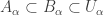 . Since is countable, there is some
  such that
  is uncountable. It follows that for any finite
  ,
, ![\bigcap \limits_{\alpha \in E} [A_\alpha,U_\alpha] \ne \varnothing](https://s0.wp.com/latex.php?latex=%5Cbigcap+%5Climits_%7B%5Calpha+%5Cin+E%7D+%5BA_%5Calpha%2CU_%5Calpha%5D+%5Cne+%5Cvarnothing&bg=ffffff&fg=333333&s=0&c=20201002) .
.
Thus if the ground space has a countable network, then has the CCC.
__________________________________
The implications in bullet points 12 and 13 cannot be reversed. Hereditarily Lindelof property and hereditarily separability are not sufficient conditions for to have the CCC. See [4] for a study of the CCC property of the Pixley-Roy spaces.
To see bullet point 15, let  be the Sorgenfrey line, i.e. the real line
  with the topology generated by the half closed intervals of the form
  . For each
  , let
, let  . Then
 ![\left\{[ \left\{ x \right\},U_x]: x \in S \right\}](https://s0.wp.com/latex.php?latex=%5Cleft%5C%7B%5B+%5Cleft%5C%7B+x+%5Cright%5C%7D%2CU_x%5D%3A+x+%5Cin+S+%5Cright%5C%7D&bg=ffffff&fg=333333&s=0&c=20201002) is a collection of pairwise disjoint open sets in
is a collection of pairwise disjoint open sets in ![\mathcal{F}[S]](https://s0.wp.com/latex.php?latex=%5Cmathcal%7BF%7D%5BS%5D&bg=ffffff&fg=333333&s=0&c=20201002) .
.
__________________________________
A Moore space is a space with a development. For the definition, see this previous post.
To see bullet point 16, for each , let  be a decreasing local base at . We define a development for the space .
For each finite  and for each , let
  . Clearly, the sets
  form a decreasing local base at the finite set . For each , let
  be the following collection:
We claim that  is a development for . To this end, let be open in with
  . If we make large enough, we have
 ![[F,B_n(F)] \subset V](https://s0.wp.com/latex.php?latex=%5BF%2CB_n%28F%29%5D+%5Csubset+V&bg=ffffff&fg=333333&s=0&c=20201002) .
.
For each non-empty proper  , choose an integer
  such that
 ![[F,B_{f(G)}(F)] \subset V](https://s0.wp.com/latex.php?latex=%5BF%2CB_%7Bf%28G%29%7D%28F%29%5D+%5Csubset+V&bg=ffffff&fg=333333&s=0&c=20201002) and
and  . Let
. Let  be defined by:
We have  for all non-empty proper . Thus
 ![F \notin [G,B_m(G)]](https://s0.wp.com/latex.php?latex=F+%5Cnotin+%5BG%2CB_m%28G%29%5D&bg=ffffff&fg=333333&s=0&c=20201002) for all non-empty proper . But in
for all non-empty proper . But in  , the only sets that contain are
 ![[F,B_m(F)]](https://s0.wp.com/latex.php?latex=%5BF%2CB_m%28F%29%5D&bg=ffffff&fg=333333&s=0&c=20201002) and
and ![[G,B_m(G)]](https://s0.wp.com/latex.php?latex=%5BG%2CB_m%28G%29%5D&bg=ffffff&fg=333333&s=0&c=20201002) for all non-empty proper . So is the only set in that contains , and clearly
for all non-empty proper . So is the only set in that contains , and clearly ![[F,B_m(F)] \subset V](https://s0.wp.com/latex.php?latex=%5BF%2CB_m%28F%29%5D+%5Csubset+V&bg=ffffff&fg=333333&s=0&c=20201002) .
.
We have shown that for each open in with , there exists an such that any open set in that contains must be a subset of . This shows that the defined above form a development for .
____________________________________________________________________
Examples
In the original construction of Pixley and Roy, the example was ![\mathcal{F}[\mathbb{R}]](https://s0.wp.com/latex.php?latex=%5Cmathcal%7BF%7D%5B%5Cmathbb%7BR%7D%5D&bg=ffffff&fg=333333&s=0&c=20201002) . Based on the above discussion, is a non-separable CCC Moore space. Because the density (greater than
. Based on the above discussion, is a non-separable CCC Moore space. Because the density (greater than  for not separable) and the cellularity (
 for CCC) do not agree, is not metrizable. In fact, it does not even have a dense metrizable subspace. Note that countable subspaces of are metrizable but are not dense. Any uncountable dense subspace of is not separable but has the CCC. Not only is not metrizable, it is not normal. The problem of finding
  for which is normal requires extra set-theoretic axioms beyond ZFC (see [6]). In fact, Pixley-Roy spaces played a large role in the normal Moore space conjecture. Assuming some extra set theory beyond ZFC, there is a subset
  such that
 ![\mathcal{F}[M]](https://s0.wp.com/latex.php?latex=%5Cmathcal%7BF%7D%5BM%5D&bg=ffffff&fg=333333&s=0&c=20201002) is a CCC metacompact normal Moore space that is not metrizable (see Example I in [8]).
is a CCC metacompact normal Moore space that is not metrizable (see Example I in [8]).
On the other hand, Pixley-Roy space of the Sorgenfrey line and the Pixley-Roy space of (the first uncountable ordinal with the order topology) are metrizable (see [3]).
The Sorgenfrey line and the first uncountable ordinal are classic examples of topological spaces that demonstrate that topological spaces in general are not as well behaved like metrizable spaces. Yet their Pixley-Roy spaces are nice. The real line and other separable metric spaces are nice spaces that behave well. Yet their Pixley-Roy spaces are very much unlike the ground spaces. This inverse relation between the ground space and the Pixley-Roy space was noted by van Douwen (see [3] and [7]) and is one reason that Pixley-Roy hyperspaces are a good source of counterexamples.
____________________________________________________________________
Reference
- Bennett, H. R., Fleissner, W. G., Lutzer, D. J., Metrizability of certain Pixley-Roy spaces, Fund. Math. 110, 51-61, 1980.
- Daniels, P, Pixley-Roy Spaces Over Subsets of the Reals, Topology Appl. 29, 93-106, 1988.
- Lutzer, D. J., Pixley-Roy topology, Topology Proc. 3, 139-158, 1978.
- Hajnal, A., Juahasz, I., When is a Pixley-Roy Hyperspace CCC?, Topology Appl. 13, 33-41, 1982.
- Pixley, C., Roy, P., Uncompletable Moore spaces, Proc. Auburn Univ. Conf. Auburn, AL, 1969.
- Przymusinski, T., Normality and paracompactness of Pixley-Roy hyperspaces, Fund. Math. 113, 291-297, 1981.
- van Douwen, E. K., The Pixley-Roy topology on spaces of subsets, Set-theoretic Topology, Academic Press, New York, 111-134, 1977.
- Tall, F. D., Normality versus Collectionwise Normality, Handbook of Set-Theoretic Topology (K. Kunen and J. E. Vaughan, eds), Elsevier Science Publishers B. V., Amsterdam, 685-732, 1984.
- Tanaka, H, Normality and hereditary countable paracompactness of Pixley-Roy hyperspaces, Fund. Math. 126, 201-208, 1986.
____________________________________________________________________


![D=[0,1] \times \{ 0,1 \}](https://s0.wp.com/latex.php?latex=D%3D%5B0%2C1%5D+%5Ctimes+%5C%7B+0%2C1+%5C%7D&bg=ffffff&fg=333333&s=0&c=20201002)


![\displaystyle \biggl[ [a,b) \times \{ 1 \} \biggr] \cup \biggl[ (a,b) \times \{ 0 \} \biggr]](https://s0.wp.com/latex.php?latex=%5Cdisplaystyle+%5Cbiggl%5B+%5Ba%2Cb%29+%5Ctimes+%5C%7B+1+%5C%7D+%5Cbiggr%5D+%5Ccup+%5Cbiggl%5B+%28a%2Cb%29+%5Ctimes+%5C%7B+0+%5C%7D+%5Cbiggr%5D&bg=ffffff&fg=333333&s=0&c=20201002)


![\biggl[ (c,a) \times \{ 1 \} \biggr] \cup \biggl[ (c,a] \times \{ 0 \} \biggr]](https://s0.wp.com/latex.php?latex=%5Cbiggl%5B+%28c%2Ca%29+%5Ctimes+%5C%7B+1+%5C%7D+%5Cbiggr%5D+%5Ccup+%5Cbiggl%5B+%28c%2Ca%5D+%5Ctimes+%5C%7B+0+%5C%7D+%5Cbiggr%5D&bg=ffffff&fg=333333&s=0&c=20201002)


![[0,1]](https://s0.wp.com/latex.php?latex=%5B0%2C1%5D&bg=ffffff&fg=333333&s=0&c=20201002)


![[-1,1]](https://s0.wp.com/latex.php?latex=%5B-1%2C1%5D&bg=ffffff&fg=333333&s=0&c=20201002)


![(a,1] \times \{ 0 \}](https://s0.wp.com/latex.php?latex=%28a%2C1%5D+%5Ctimes+%5C%7B+0+%5C%7D&bg=ffffff&fg=333333&s=0&c=20201002)


![(0,a] \times \{ 0 \}](https://s0.wp.com/latex.php?latex=%280%2Ca%5D+%5Ctimes+%5C%7B+0+%5C%7D&bg=ffffff&fg=333333&s=0&c=20201002)
![\displaystyle U_a(y) = \left\{ \begin{array}{ll} \displaystyle 1 &\ \ \ \ \ \ y \in [a,1) \times \{ 1 \} \\ \text{ } & \text{ } \\ \displaystyle 1 &\ \ \ \ \ \ y \in (a,1] \times \{ 0 \} \\ \text{ } & \text{ } \\ 0 &\ \ \ \ \ \ y \in (0,a] \times \{ 0 \} \\ \text{ } & \text{ } \\ 0 &\ \ \ \ \ \ y \in [0,a) \times \{ 1 \} \\ \text{ } & \text{ } \\ 0 &\ \ \ \ \ \ y=(0,0) \text{ or } y = (1,1) \end{array} \right.](https://s0.wp.com/latex.php?latex=%5Cdisplaystyle++U_a%28y%29+%3D+%5Cleft%5C%7B+%5Cbegin%7Barray%7D%7Bll%7D+++++++++++%5Cdisplaystyle++1+%26%5C+%5C+%5C+%5C+%5C+%5C+y+%5Cin+%5Ba%2C1%29+%5Ctimes+%5C%7B+1+%5C%7D+%5C%5C++++++++++++%5Ctext%7B+%7D+%26+%5Ctext%7B+%7D+%5C%5C++++++++++%5Cdisplaystyle++1+%26%5C+%5C+%5C+%5C+%5C+%5C+y+%5Cin+%28a%2C1%5D+%5Ctimes+%5C%7B+0+%5C%7D+%5C%5C+++++++++++%5Ctext%7B+%7D+%26+%5Ctext%7B+%7D+%5C%5C+++++++++++0+%26%5C+%5C+%5C+%5C+%5C+%5C+y+%5Cin+%280%2Ca%5D+%5Ctimes+%5C%7B+0+%5C%7D+%5C%5C+++++++++++%5Ctext%7B+%7D+%26+%5Ctext%7B+%7D+%5C%5C+++++++++++0+%26%5C+%5C+%5C+%5C+%5C+%5C+y+%5Cin+%5B0%2Ca%29+%5Ctimes+%5C%7B+1+%5C%7D+%5C%5C+++++++++++%5Ctext%7B+%7D+%26+%5Ctext%7B+%7D+%5C%5C+++++++++++0+%26%5C+%5C+%5C+%5C+%5C+%5C+y%3D%280%2C0%29+%5Ctext%7B+or+%7D+y+%3D+%281%2C1%29+++++++++++%5Cend%7Barray%7D+%5Cright.&bg=ffffff&fg=333333&s=0&c=20201002)


-Theory Problem Book, Topological and Function Spaces, Springer, New York, 2011.


 . The union of such open intervals is called an open set. If more than one topologies are considered on the real line, these open sets are referred to as the usual open sets or Euclidean open sets (on the real line). The open intervals
  form a base for the usual topology on the real line. One important fact abut the usual open sets is that the usual open sets can be generated by the intervals
  open intervals. Then form open sets by taking unions of all such open intervals. The collection of such open sets is called the Sorgenfrey topology (on the real line). The real number line
  . The Sorgenfrey line has been discussed in this blog, starting with
  . Thus any usual (Euclidean) open set is an open set in the Sorgenfrey line. Thus the usual topology (on the real line) is contained in the Sorgenfrey topology, i.e. the usual topology is a weaker (coarser) topology.
 be the set of all continuous functions
  where the domain is the real number line with the usual topology. Let
  be the set of all continuous functions
  where the domain is the Sorgenfrey line. In both cases, the range is always the number line with the usual topology. Based on the preceding paragraph, any continuous function
  .
.

 where
where  . Both of these are continuous in the usual Euclidean topology (in the domain). Such graphs would make regular appearance in a course on probability and statistics. They also show up in a calculus course as an everywhere differentiable curve (Figure 1) and as a differentiable curve except at finitely many points (Figure 2). Both of these functions can also be regarded as continuous functions on the Sorgenfrey line.
 to -1 and maps the interval
  to 1. It is not continuous in the usual topology because of the jump at
  . But it is a continuous function when the domain is considered to be the Sorgenfrey line. Because of the open intervals being
 , where each point has probability 0.2. There is a jump of height 0.2 at each of the points from 0 to 4. Figure 3 and Figure 4 are step functions. As long as the left point of a step is solid and the right point is hollow, the step functions are continuous on the Sorgenfrey line.
 for
for 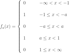
 . So we can consider
  . See
. See  , and for any open interval
 ![[x,(a,b)]=\left\{h \in C_p(\mathbb{S}): h(x) \in (a, b) \right\}](https://s0.wp.com/latex.php?latex=%5Bx%2C%28a%2Cb%29%5D%3D%5Cleft%5C%7Bh+%5Cin+C_p%28%5Cmathbb%7BS%7D%29%3A+h%28x%29+%5Cin+%28a%2C+b%29+%5Cright%5C%7D&bg=ffffff&fg=333333&s=0&c=20201002) . Then the collection of intersections of finitely many
. Then the collection of intersections of finitely many ![[x,(a,b)]](https://s0.wp.com/latex.php?latex=%5Bx%2C%28a%2Cb%29%5D&bg=ffffff&fg=333333&s=0&c=20201002) would form a base for
would form a base for 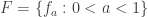 is a closed and discrete subspace of
 containing
  for any
  . To this end, let
 ![O=[a,V_1] \cap [-a,V_2]](https://s0.wp.com/latex.php?latex=O%3D%5Ba%2CV_1%5D+%5Ccap+%5B-a%2CV_2%5D&bg=ffffff&fg=333333&s=0&c=20201002) where
where  and
and  are the open intervals
  and
and  . With Figure 6 as an aid, it follows that for
  ,
,  and for
  ,
,  .
.  and
and  . Thus
  and
and  . Thus
  , there is an open set
  such that
  . As we consider
  such that
  .
.  and
and  . Then for all
  and for all
  . Let
. Let ![U=[a,(-0.1,0.1)] \cap [-a,(0.9,1.1)]](https://s0.wp.com/latex.php?latex=U%3D%5Ba%2C%28-0.1%2C0.1%29%5D+%5Ccap+%5B-a%2C%280.9%2C1.1%29%5D&bg=ffffff&fg=333333&s=0&c=20201002) . Then
. Then  and
and  for any
  for any
  and
and  has a similar argument.
 .
.  . Suppose not. Let
  such that
  . Suppose that
 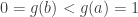 . Consider
  . Clearly the number
  . Let
. Let  be a least upper bound of
  . Otherwise,
  would not be the least upper bound of the set
  in the interval
  such that
  from the left such that
  for all
  . Otherwise, the function
  . By the assumption in Case 2,
  and
and 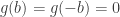 . Since
  for all
  from the right. Since
  , contradicting
  . Thus we cannot have
  where
where  . Clearly
  for all
  . Otherwise, the function
  and
and  . Since
  for all
 ![U=[0,(0.9,1.1)]](https://s0.wp.com/latex.php?latex=U%3D%5B0%2C%280.9%2C1.1%29%5D&bg=ffffff&fg=333333&s=0&c=20201002) . It is clear that
. It is clear that  . Let
. Let ![U=[-1,(-0.1,0.1)]](https://s0.wp.com/latex.php?latex=U%3D%5B-1%2C%28-0.1%2C0.1%29%5D&bg=ffffff&fg=333333&s=0&c=20201002) . It is clear that
. It is clear that  , then
  , the space of real-valued continuous functions defined on the number line with the pointwise convergence topology, is hereditarily separable and thus separable. Recall that continuous functions in
  of a space
  subset of
  subset of
  is a
is a  and
and  of
of  and
and  of
of  and
and  . A space
  and
and  of
of  and
and  . Clearly any normal space is subnormal. The Sorgenfrey plane is an example of a subnormal space that is not normal.
  show that these two weak forms of normality (pseudonormal and subnormal) are not equivalent. The space
  . The Sorgenfrey plane is the product space
  be the interior of
 where each
  . We claim that
  ,
,  for some
  . Note that
  , which means that no point of the open interval
  can belong to
  for some
  , a contradiction. Thus
 is perfect.
 such that each
  , in addition to being a collection of basic open sets, is a discrete collection. The existence of such a base is equivalent to metrizability, a well known result called Bing’s metrization theorem (see Theorem 4.4.8 in [1]). Let
  such that
  and
and  . Thus
  . Thus we have:
 be defined by
 , let
, let  where each
  is a closed subset of
  by
by
 . Since
  is discrete, there exists some open subset
  of
of  such that
  where
where  . Then
  is an open subset of
  such that
  . Then
  is a closed subset of
  over all countably many possible pairs
  . Thus
  and
and  where
where  and
and  are perfect. Also note that the Sorgenfrey plane topology is finer than the topologies for both
  . Consider the sets
  and
and  defined by:

 . We claim that
  , and for each positive integer
  , let
, let  be the half-open square
  . Then
  is a local base at the point
  by
by
 . We claim that each
  . In relation to the point


 , it follows that
  . We show that for each of these three sets, there is an open set containing the point
  . If
. If  . Let
. Let  . Note that
  and
and  . Now consider the following open set:
 is an open set containing the point
  . Suppose
  . Then
  and
and  . Consider the following set:
 , it follows that
  . Thus
  . It follows that
  since
since

 . Hence
  , a contradiction. Thus the claim that
  is symmetrical to the case
  . If
. If  . Let
. Let  . Note that
  and
and 
 . Suppose
  . Then
  and
and 
 . Thus the claim that
  is perfect, then
  is perfect. We take the inductive proof in [2] and adapt it for the Sorgenfrey plane. The authors in [2] also proved that for a sequence of spaces
  such that the product of any finite number of these spaces is perfect, the product
  is perfect. Then
  is perfect.
 with the order topology. Let
  be the disjoint sum (union) of
  , we can always separate the disjoint closed sets
  such that
  . For each real number


 is the vertical line of height 2 at the point
  . The set
  is the line originating at
 ")
 where
where  is isolated.
 , a basic open set is of the form
  where
where  and
and  .
.

 where
where  is finite and
  . Furthermore, break up
  by letting
  and
and  . Let
. Let 
 .
. by
by  . Let
. Let 

 . Choose
  on the left of
  and
and  . This means that
 .
.
 . In this post, we use
  is a closed and discrete set and is called the anti-diagonal. The proof presented in

 . The points lying above the x-axis have the usual Euclidean open neighborhoods. A point
  together with the interior of a disc in the upper half plane that is tangent at the point

 . The second factor is the successor ordinal to
  to denote this space.
  as a subspace of
  (
( for some ordinal
  ) such that
  . Based on the discussion in the preceding paragraph, there are disjoint open sets
  and
and  in
in  such that
  and
and  . With
  being a successor ordinal, the square

 with
with  ,
,  is normal but not paracompact (see Example 6.3 in [1] and see [3]). Even though
  be the space defined as in Example 3 above except that only points of
 ![[F,U]=\left\{B \in \mathcal{F}[X]: F \subset B \subset U \right\}](https://s0.wp.com/latex.php?latex=%5BF%2CU%5D%3D%5Cleft%5C%7BB+%5Cin+%5Cmathcal%7BF%7D%5BX%5D%3A+F+%5Csubset+B+%5Csubset+U+%5Cright%5C%7D&bg=ffffff&fg=333333&s=0&c=20201002)
![H_n=\left\{F \in \mathcal{F}[X]: x \in F \text{ and } \lvert F \lvert \le n \right\}](https://s0.wp.com/latex.php?latex=H_n%3D%5Cleft%5C%7BF+%5Cin+%5Cmathcal%7BF%7D%5BX%5D%3A+x+%5Cin+F+%5Ctext%7B+and+%7D+%5Clvert+F+%5Clvert+%5Cle+n+%5Cright%5C%7D&bg=ffffff&fg=333333&s=0&c=20201002)
![D=\bigcup \left\{A: [A,U] \in \mathcal{G} \text{ for some open } U \right\}](https://s0.wp.com/latex.php?latex=D%3D%5Cbigcup+%5Cleft%5C%7BA%3A+%5BA%2CU%5D+%5Cin+%5Cmathcal%7BG%7D+%5Ctext%7B+for+some+open+%7D+U++%5Cright%5C%7D&bg=ffffff&fg=333333&s=0&c=20201002)
![\mathcal{H}_n=\left\{[F,B_n(F)]: F \in \mathcal{F}[X] \right\}](https://s0.wp.com/latex.php?latex=%5Cmathcal%7BH%7D_n%3D%5Cleft%5C%7B%5BF%2CB_n%28F%29%5D%3A+F+%5Cin+%5Cmathcal%7BF%7D%5BX%5D+%5Cright%5C%7D&bg=ffffff&fg=333333&s=0&c=20201002)

 where the topology is generated by a base consisting the half open intervals of the form
  of open covers of
  satisfying the condition that for any open set
  ,
,  . When
  . Thus metric spaces are developable. There are plenty of non-metrizable Moore space. One example is the
  is a
is a  is a countable base for
  -locally finite base for
  of closed sets in
  of open subsets of
  . For a proof of Bing’s metrization theorem, see page 329 of [1].


 , see
, see  , see
, see  . All spaces considered here are at least Tychonoff (i.e. completely regular). For any basic notions not defined here, see [1] or [2].
 .
. is submetrizable if there is another topology
  that can be defined on
  and
and  is metrizable. The Sorgenfrey line is non-metrizable and yet the Sorgenfrey topology has a weaker topology that is metrizable, namely the Euclidean topology of the real line.
 is a locally finite family of non-empty open subsets of
 does not hold. Then there is an infinite locally finite family of non-empty open sets
  . We wish to define an unbounded continuous function using
  . Then for each
 ![f_n:X \rightarrow [0,n]](https://s0.wp.com/latex.php?latex=f_n%3AX+%5Crightarrow+%5B0%2Cn%5D&bg=ffffff&fg=333333&s=0&c=20201002) such that
such that  and
and  . Define
  by
by  .
.  . In other words, for each
  ,
,  for all
  . Thus the function
  ,
,  , showing that it is unbounded.
 and
and  are clear.
 be a continuous function. We want to show that
  where each
  . Note that
  ,
,  is a family of non-empty open subsets of
  for each
  .
. .
. for all
  , then we are done. So assume that
  are distinct for infinitely many
  for infinitely many
  .
. . Then let
  ,
,  ,
,  , and so on. By condition
 . Clearly the open sets
  have the finite intersection property. Because
  .
.  . The interior of
  , is the set of all points
  . Points of
  is said to be a closed domain if
  . It is clear that
  is pseudocompact for any nonempty open set
  . Let
. Let  where
where  be a decreasing sequence of open subsets of
  contains points of the open set
  for each
  . Note that the open sets
  form a decreasing sequence of open sets in the pseudocompact space
  are also points in
  (closure with respect to
  , leading to the conclusion that
  and the closure of
  .
. is also a closed set with respect to the topology
  . We make the following claims.
 .
. is pseudocompact in
  . The reverse set inclusion follows from the fact that
  are closed domains in the pseudocompact space
  .
. .
. be the set of all continuous real-valued functions defined on the space
 says that there are at least as many continuous real-valued functions as there are subsets of the closed and discrete set
  ,
,  are disjoint closed sets in
 ![f_E:X \rightarrow [0,1]](https://s0.wp.com/latex.php?latex=f_E%3AX+%5Crightarrow+%5B0%2C1%5D&bg=ffffff&fg=333333&s=0&c=20201002) such that
such that  maps
maps  and
and  . Note that the mapping
  defined by
  is a one-to-one map, where
  is the collection of all subsets of
  defined by
  , which is the function
  refers to the set of all functions from the set
  and
and  ), then
  on the whole space
  is a one-to-one map. Some elementary cardinal arithmetic shows that
  . Thus the second inequality in
  where
where  . For any separable space
  . If the space
  such that every closed and discrete set in
  . The extent of the space
  . For more detailed information about cardinal functions, see [2].
 .
. , which implies
  .
. is an upper bound of the cardinalities of closed and discrete sets in any normal space
  be a space with at least two points. For each
  . Then the product space
  contains a discrete subspace
  by the following:
 . It follows that
  and that
 ![[0,1]^{\omega_1}](https://s0.wp.com/latex.php?latex=%5B0%2C1%5D%5E%7B%5Comega_1%7D&bg=ffffff&fg=333333&s=0&c=20201002) , the product of
, the product of  , the product of
 and let
 ![X_\alpha=[0,1]](https://s0.wp.com/latex.php?latex=X_%5Calpha%3D%5B0%2C1%5D&bg=ffffff&fg=333333&s=0&c=20201002) for all
for all  . Then the product space
  with
with  , by the open interval
  . Let
. Let  . A set
  is said to be a closed set if the complement
  is an open set.
 is an open set. Note that it is the union of two open intervals. The set of all positive numbers
  is open. Note that
  .
.  are open sets.
 ,
,  ,
,  ,
,  ,
,  is obviously not an open set in the real line. However
  , is an open set in the space
 (i.e. the set of all rational bumbers
 ![(a,1]=[0,1] \cap (a,b)](https://s0.wp.com/latex.php?latex=%28a%2C1%5D%3D%5B0%2C1%5D+%5Ccap+%28a%2Cb%29&bg=ffffff&fg=333333&s=0&c=20201002) where
where  . Likewise, an open interval containing the left endpoint
  . In general, for the subset
  . The set of all open sets just defined for the subset
  -defintion is used. We consider continuous functions from a topological point of view.
![[1]](https://s0.wp.com/latex.php?latex=%5B1%5D&bg=ffffff&fg=333333&s=0&c=20201002) . The function
. The function  is continuous at
  if
if  . For the definition of
  , we have the following from
  is the limit of
  as
as  , there exists a number
  such that
  for all
  .
. be a function. The function
  , there is some open interval
  containing
  . The function
  corresponds to the
  in definition
  is the
  in definition
  , the inverse image
  is an open set in the domain space
  is a closed set in the domain space
  and
and  as well as exponential functions such as
  and logarithmic functions such as
  .
.
 is not continuous at every
  .
.
 . Define
  by
by  . The function
  is continuous at every
  . Theorem
  be the set of all open sets generated by the open intervals
  ). To see this, for each
  , we have
  where
where  . Thus
  being the distance between
  where
where  is the collection of all open sets, which is called a topology. In our first example,
  is the set of all open sets generated by the open intervals
  is the set of all open sets generated by the open intervals
  satisfies the same three conditions stated in Theorem
  and
and  , then there is some
  such that
  and
and  .
.![[2]](https://s0.wp.com/latex.php?latex=%5B2%5D&bg=ffffff&fg=333333&s=0&c=20201002) ).
).