Countably paracompact spaces

Posted on December 8, 2016 by Dan Ma

This post is a basic discussion on countably paracompact space. A space is a paracompact space if every open cover has a locally finite open refinement. The definition can be tweaked by saying that only open covers of size not more than a certain cardinal number $\tau$ can have a locally finite open refinement (any space with this property is called a $\tau$ -paracompact space). The focus here is that the open covers of interest are countable in size. Specifically, a space is a countably paracompact space if every countable open cover has a locally finite open refinement. Even though the property appears to be weaker than paracompact spaces, the notion of countably paracompactness is important in general topology. This post discusses basic properties of such spaces. All spaces under consideration are Hausdorff.

Basic discussion of paracompact spaces and their Cartesian products are discussed in these two posts (here and here).

A related notion is that of metacompactness. A space is a metacompact space if every open cover has a point-finite open refinement. For a given open cover, any locally finite refinement is a point-finite refinement. Thus paracompactness implies metacompactness. The countable version of metacompactness is also interesting. A space is countably metacompact if every countable open cover has a point-finite open refinement. In fact, for any normal space, the space is countably paracompact if and only of it is countably metacompact (see Corollary 2 below).

____________________________________________________________________

Normal Countably Paracompact Spaces

A good place to begin is to look at countably paracompactness along with normality. In 1951, C. H. Dowker characterized countably paracompactness in the class of normal spaces.

Theorem 1 (Dowker’s Theorem)
Let $X$ be a normal space. The following conditions are equivalent.

The space $X$ is countably paracompact.
Every countable open cover of $X$ has a point-finite open refinement.
If $\left\{U_n: n=1,2,3,\cdots \right\}$ is an open cover of $X$ , there exists an open refinement $\left\{V_n: n=1,2,3,\cdots \right\}$ such that $\overline{V_n} \subset U_n$ for each $n$ .
The product space $X \times Y$ is normal for any compact metric space $Y$ .
The product space $X \times [0,1]$ is normal where $[0,1]$ is the closed unit interval with the usual Euclidean topology.
For each sequence $\left\{A_n \subset X: n=1,2,3,\cdots \right\}$ of closed subsets of $X$ such that $A_1 \supset A_2 \supset A_3 \supset \cdots$ and $\cap_n A_n=\varnothing$ , there exist open sets $B_1,B_2,B_3,\cdots$ such that $A_n \subset B_n$ for each $n$ such that $\cap_n B_n=\varnothing$ .

Dowker’s Theorem is proved in this previous post. Condition 2 in the above formulation of the Dowker’s theorem is not in the Dowker’s theorem in the previous post. In the proof for $1 \rightarrow 2$ in the previous post is essentially $1 \rightarrow 2 \rightarrow 3$ for Theorem 1 above. As a result, we have the following.

Corollary 2
Let $X$ be a normal space. Then $X$ is countably paracompact if and only of $X$ is countably metacompact.

Theorem 1 indicates that normal countably paracompact spaces are important for the discussion of normality in product spaces. As a result of this theorem, we know that normal countably paracompact spaces are productively normal with compact metric spaces. The Cartesian product of normal spaces with compact spaces can be non-normal (an example is found here). When the normal factor is countably paracompact and the compact factor is upgraded to a metric space, the product is always normal. The connection with normality in products is further demonstrated by the following corollary of Theorem 1.

Corollary 3
Let $X$ be a normal space. Let $Y$ be a non-discrete metric space. If $X \times Y$ is normal, then $X$ is countably paracompact.

Since $Y$ is non-discrete, there is a non-trivial convergent sequence (i.e. the sequence represents infinitely many points). Then the sequence along with the limit point is a compact metric subspace of $Y$ . Let’s call this subspace $S$ . Then $X \times S$ is a closed subspace of the normal $X \times Y$ . As a result, $X \times S$ is normal. By Theorem 1, $X$ is countably paracompact.

C. H. Dowker in 1951 raised the question: is every normal space countably paracompact? Put it in another way, is the product of a normal space and the unit interval always a normal space? As a result of Theorem 1, any normal space that is not countably paracompact is called a Dowker space. The search for a Dowker space took about 20 years. In 1955, M. E. Rudin showed that a Dowker space can be constructed from assuming a Souslin line. In the mid 1960s, the existence of a Souslin line was shown to be independent of the usual axioms of set theorey (ZFC). Thus the existence of a Dowker space was known to be consistent with ZFC. In 1971, Rudin constructed a Dowker space in ZFC. Rudin’s Dowker space has large cardinality and is pathological in many ways. Zoltan Balogh constructed a small Dowker space (cardinality continuum) in 1996. Various Dowker space with nicer properties have also been constructed using extra set theory axioms. The first ZFC Dowker space constructed by Rudin is found in [2]. An in-depth discussion of Dowker spaces is found in [3]. Other references on Dowker spaces is found in [4].

Since Dowker spaces are rare and are difficult to come by, we can employ a “probabilistic” argument. For example, any “concrete” normal space (i.e. normality can be shown without using extra set theory axioms) is likely to be countably paracompact. Thus any space that is normal and not paracompact is likely countably paracompact (if the fact of being normal and not paracompact is established in ZFC). Indeed, any well known ZFC example of normal and not paracompact must be countably paracompact. In the long search for Dowker spaces, researchers must have checked all the well known examples! This probability thinking is not meant to be a proof that a given normal space is countably paracompact. It is just a way to suggest a possible answer. In fact, a good exercise is to pick a normal and non-paracompact space and show that it is countably paracompact.

____________________________________________________________________

Some Examples

The following lists out a few classes of spaces that are always countably paracompact.

Metric spaces are countably paracompact.
Paracompact spaces are countably paracompact.
Compact spaces are countably paracompact.
Countably compact spaces are countably paracompact.
Perfectly normal spaces are countably paracompact.
Normal Moore spaces are countably paracompact.
Linearly ordered spaces are countably paracompact.
Shrinking spaces are countably paracompact.

The first four bullet points are clear. Metric spaces are paracompact. It is clear from definition that paracompact spaces, compact and countably compact spaces are countably paracompact. One way to show perfect normal spaces are countably paracompact is to show that they satisfy condition 6 in Theorem 1 (shown here). Any Moore space is perfect (closed sets are $G_\delta$ ). Thus normal Moore space are perfectly normal and hence countably paracompact. The proof of the countably paracompactness of linearly ordered spaces can be found in [1]. See Theorem 5 and Corollary 6 below for the proof of the last bullet point.

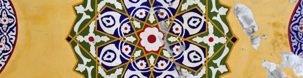
As suggested by the probability thinking in the last section, we now look at examples of countably paracompact spaces among spaces that are “normal and not paracompact”. The first uncountable ordinal $\omega_1$ is normal and not paracompact. But it is countably compact and is thus countably paracompact.

Example 1
Any $\Sigma$ -product of uncountably many metric spaces is normal and countably paracompact.

For each $\alpha<\omega_1$ , let $X_\alpha$ be a metric space that has at least two points. Assume that each $X_\alpha$ has a point that is labeled 0. Consider the following subspace of the product space $\prod_{\alpha<\omega_1} X_\alpha$ .

$\displaystyle \Sigma_{\alpha<\omega_1} X_\alpha =\left\{f \in \prod_{\alpha<\omega_1} X_\alpha: \ f(\alpha) \ne 0 \text{ for at most countably many } \alpha \right\}$

The space $\Sigma_{\alpha<\omega_1} X_\alpha$ is said to be the $\Sigma$ -product of the spaces $X_\alpha$ . It is well known that the $\Sigma$ -product of metric spaces is normal, in fact collectionwise normal (this previous post has a proof that $\Sigma$ -product of separable metric spaces is collectionwise normal). On the other hand, any $\Sigma$ -product always contains $\omega_1$ as a closed subset as long as there are uncountably many factors and each factor has at least two points (see the lemma in this previous post). Thus any such $\Sigma$ -product, including the one being discussed, cannot be paracompact.

Next we show that $T=(\Sigma_{\alpha<\omega_1} X_\alpha) \times [0,1]$ is normal. The space $T$ can be reformulated as a $\Sigma$ -product of metric spaces and is thus normal. Note that $T=\Sigma_{\alpha<\omega_1} Y_\alpha$ where $Y_0=[0,1]$ , for any $n$ with $1 \le n<\omega$ , $Y_n=X_{n-1}$ and for any $\alpha$ with $\alpha>\omega$ , $Y_\alpha=X_\alpha$ . Thus $T$ is normal since it is the $\Sigma$ -product of metric spaces. By Theorem 1, the space $\Sigma_{\alpha<\omega_1} X_\alpha$ is countably paracompact. $\square$

Example 2
Let $\tau$ be any uncountable cardinal number. Let $D_\tau$ be the discrete space of cardinality $\tau$ . Let $L_\tau$ be the one-point Lindelofication of $D_\tau$ . This means that $L_\tau=D_\tau \cup \left\{\infty \right\}$ where $\infty$ is a point not in $D_\tau$ . In the topology for $L_\tau$ , points in $D_\tau$ are isolated as before and open neighborhoods at $\infty$ are of the form $L_\tau - C$ where $C$ is any countable subset of $D_\tau$ . Now consider $C_p(L_\tau)$ , the space of real-valued continuous functions defined on $L_\tau$ endowed with the pointwise convergence topology. The space $C_p(L_\tau)$ is normal and not Lindelof, hence not paracompact (discussed here). The space $C_p(L_\tau)$ is also homeomorphic to a $\Sigma$ -product of $\tau$ many copies of the real lines. By the same discussion in Example 1, $C_p(L_\tau)$ is countably paracompact. For the purpose at hand, Example 2 is similar to Example 1. $\square$

Example 3
Consider R. H. Bing’s example G, which is a classic example of a normal and not collectionwise normal space. It is also countably paracompact. This previous post shows that Bing’s Example G is countably metacompact. By Corollary 2, it is countably paracompact. $\square$

Based on the “probabilistic” reasoning discussed at the end of the last section (based on the idea that Dowker spaces are rare), “normal countably paracompact and not paracompact” should be in plentiful supply. The above three examples are a small demonstration of this phenomenon.

Existence of Dowker spaces shows that normality by itself does not imply countably paracompactness. On the other hand, paracompact implies countably paracompact. Is there some intermediate property that always implies countably paracompactness? We point that even though collectionwise normality is intermediate between paracompactness and normality, it is not sufficiently strong to imply countably paracompactness. In fact, the Dowker space constructed by Rudin in 1971 is collectionwise normal.

____________________________________________________________________

More on Countably Paracompactness

Without assuming normality, the following is a characterization of countably paracompact spaces.

Theorem 4
Let $X$ be a topological space. Then the space $X$ is countably paracompact if and only of the following condition holds.

For any decreasing sequence $\left\{A_n: n=1,2,3,\cdots \right\}$ of closed subsets of $X$ such that $\cap_n A_n=\varnothing$ , there exists a decreasing sequence $\left\{B_n: n=1,2,3,\cdots \right\}$ of open subsets of $X$ such that $A_n \subset B_n$ for each $n$ and $\cap_n \overline{B_n}=\varnothing$ .

Proof of Theorem 4
Suppose that $X$ is countably paracompact. Suppose that $\left\{A_n: n=1,2,3,\cdots \right\}$ is a decreasing sequence of closed subsets of $X$ as in the condition in the theorem. Then $\mathcal{U}=\left\{X-A_n: n=1,2,3,\cdots \right\}$ is an open cover of $X$ . Let $\mathcal{V}$ be a locally finite open refinement of $\mathcal{U}$ . For each $n=1,2,3,\cdots$ , define the following:

$B_n=\cup \left\{V \in \mathcal{V}: V \cap A_n \ne \varnothing \right\}$

It is clear that $A_n \subset B_n$ for each $n$ . The open sets $B_n$ are decreasing, i.e. $B_1 \supset B_2 \supset \cdots$ since the closed sets $A_n$ are decreasing. To show that $\cap_n \overline{B_n}=\varnothing$ , let $x \in X$ . The goal is to find $B_j$ such that $x \notin \overline{B_j}$ . Once $B_j$ is found, we will obtain an open set $V$ such that $x \in V$ and $V$ contains no points of $B_j$ .

Since $\mathcal{V}$ is locally finite, there exists an open set $V$ such that $x \in V$ and $V$ meets only finitely many sets in $\mathcal{V}$ . Suppose that these finitely many open sets in $\mathcal{V}$ are $V_1,V_2,\cdots,V_m$ . Observe that for each $i=1,2,\cdots,m$ , there is some $j(i)$ such that $V_i \cap A_{j(i)}=\varnothing$ (i.e. $V_i \subset X-A_{j(i)}$ ). This follows from the fact that $\mathcal{V}$ is a refinement $\mathcal{U}$ . Let $j$ be the maximum of all $j(i)$ where $i=1,2,\cdots,m$ . Then $V_i \cap A_{j}=\varnothing$ for all $i=1,2,\cdots,m$ . It follows that the open set $V$ contains no points of $B_j$ . Thus $x \notin \overline{B_j}$ .

For the other direction, suppose that the space $X$ satisfies the condition given in the theorem. Let $\mathcal{U}=\left\{U_n: n=1,2,3,\cdots \right\}$ be an open cover of $X$ . For each $n$ , define $A_n$ as follows:

$A_n=X-U_1 \cup U_2 \cup \cdots \cup U_n$

Then the closed sets $A_n$ form a decreasing sequence of closed sets with empty intersection. Let $B_n$ be decreasing open sets such that $\bigcap_{i=1}^\infty \overline{B_i}=\varnothing$ and $A_n \subset B_n$ for each $n$ . Let $C_n=X-B_n$ for each $n$ . Then $C_n \subset \cup_{j=1}^n U_j$ . Define $V_1=U_1$ . For each $n \ge 2$ , define $V_n=U_n-\bigcup_{j=1}^{n-1}C_{j}$ . Clearly each $V_n$ is open and $V_n \subset U_n$ . It is straightforward to verify that $\mathcal{V}=\left\{V_n: n=1,2,3,\cdots \right\}$ is a cover of $X$ .

We claim that $\mathcal{V}$ is locally finite in $X$ . Let $x \in X$ . Choose the least $n$ such that $x \notin \overline{B_n}$ . Choose an open set $O$ such that $x \in O$ and $O \cap \overline{B_n}=\varnothing$ . Then $O \cap B_n=\varnothing$ and $O \subset C_n$ . This means that $O \cap V_k=\varnothing$ for all $k \ge n+1$ . Thus the open cover $\mathcal{V}$ is a locally finite refinement of $\mathcal{U}$ . $\square$

___________________________________

We present another characterization of countably paracompact spaces that involves the notion of shrinkable open covers. An open cover $\mathcal{U}$ of a space $X$ is said to be shrinkable if there exists an open cover $\mathcal{V}=\left\{V(U): U \in \mathcal{U} \right\}$ of the space $X$ such that for each $U \in \mathcal{U}$ , $\overline{V(U)} \subset U$ . If $\mathcal{U}$ is shrinkable by $\mathcal{V}$ , then we also say that $\mathcal{V}$ is a shrinking of $\mathcal{U}$ . Note that Theorem 1 involves a shrinking. Condition 3 in Theorem 1 (Dowker’s Theorem) can rephrased as: every countable open cover of $X$ has a shrinking. This for any normal countably paracompact space, every countable open cover has a shrinking (or is shrinkable).

A space $X$ is a shrinking space if every open cover of $X$ is shrinkable. Every shrinking space is a normal space. This follows from this lemma: A space $X$ is normal if and only if every point-finite open cover of $X$ is shrinkable (see here for a proof). With this lemma, it follows that every shrinking space is normal. The converse is not true. To see this we first show that any shrinking space is countably paracompact. Since any Dowker space is a normal space that is not countably paracompact, any Dowker space is an example of a normal space that is not a shrinking space. To show that any shrinking space is countably paracompact, we first prove the following characterization of countably paracompactness.

Theorem 5
Let $X$ be a space. Then $X$ is countably paracompact if and only of every countable increasing open cover of $X$ is shrinkable.

Proof of Theorem 5
Suppose that $X$ is countably paracompact. Let $\mathcal{U}=\left\{U_1,U_2,U_3,\cdots \right\}$ be an increasing open cover of $X$ . Then there exists a locally open refinement $\mathcal{V}_0$ of $\mathcal{U}$ . For each $n$ , define $V_n=\cup \left\{O \in \mathcal{V}_0: O \subset U_n \right\}$ . Then $\mathcal{V}=\left\{V_1,V_2,V_3,\cdots \right\}$ is also a locally finite refinement of $\mathcal{U}$ . For each $n$ , define

$G_n=\cup \left\{O \subset X: O \text{ is open and } \forall \ m > n, O \cap V_m=\varnothing \right\}$

Let $\mathcal{G}=\left\{G_n: n=1,2,3,\cdots \right\}$ . It follows that $G_n \subset G_m$ if $n<m$ . Then $\mathcal{G}$ is an increasing open cover of $X$ . Observe that for each $n$ , $\overline{G_n} \cap V_m=\varnothing$ for all $m > n$ . Then we have the following:

$\displaystyle \begin{aligned} \overline{G_n}&\subset X-\cup \left\{V_m: m > n \right\} \\&\subset \cup \left\{V_k: k=1,2,\cdots,n \right\} \\&\subset \cup \left\{U_k: k=1,2,\cdots,n \right\}=U_n \end{aligned}$

We have just established that $\mathcal{G}$ is a shrinking of $\mathcal{U}$ , or that $\mathcal{U}$ is shrinkable.

For the other direction, to show that $X$ is countably paracompact, we show that the condition in Theorem 4 is satisfied. Let $\left\{A_1,A_2,A_3,\cdots \right\}$ be a decreasing sequence of closed subsets of $X$ with empty intersection. Then $\mathcal{U}=\left\{U_1,U_2,U_3,\cdots \right\}$ be an open cover of $X$ where $U_n=X-A_n$ for each $n$ . By assumption, $\mathcal{U}$ is shrinkable. Let $\mathcal{V}=\left\{V_1,V_2,V_3,\cdots \right\}$ be a shrinking. We can assume that $\mathcal{V}$ is an increasing sequence of open sets.

For each $n$ , let $B_n=X-\overline{V_n}$ . We claim that $\left\{B_1,B_2,B_3,\cdots \right\}$ is a decreasing sequence of open sets that expand the closed sets $A_n$ and that $\bigcap_{n=1}^\infty \overline{B_n}=\varnothing$ . The expansion part follows from the following:

$A_n=X-U_n \subset X-\overline{V_n}=B_n$

The part about decreasing follows from:

$B_{n+1}=X-\overline{V_{n+1}} \subset X-\overline{V_n}=B_n$

We show that $\bigcap_{n=1}^\infty \overline{B_n}=\varnothing$ . To this end, let $x \in X$ . Then $x \in V_n$ for some $n$ . We claim that $x \notin \overline{B_n}$ . Suppose $x \in \overline{B_n}$ . Since $V_n$ is an open set containing $x$ , $V_n$ must contain a point of $B_n$ , say $y$ . Since $y \in B_n$ , $y \notin \overline{V_n}$ . This in turns means that $y \notin V_n$ , a contradiction. Thus we have $x \notin \overline{B_n}$ as claimed. We have established that every point of $X$ is not in $\overline{B_n}$ for some $n$ . Thus the intersection of all the $\overline{B_n}$ must be empty. We have established the condition in Theorem 4 is satisfied. Thus $X$ is countably paracompact. $\square$

Corollary 6
If $X$ is a shrinking space, then $X$ is countably paracompact.

____________________________________________________________________

Reference

Ball, B. J., Countable Paracompactness in Linearly Ordered Spaces, Proc. Amer. Math. Soc., 5, 190-192, 1954. (link)
Rudin, M. E., A Normal Space $X$ for which $X \times I$ is not Normal, Fund. Math., 73, 179-486, 1971. (link)
Rudin, M. E., Dowker Spaces, Handbook of Set-Theoretic Topology (K. Kunen and J. E. Vaughan, eds), Elsevier Science Publishers B. V., Amsterdam, (1984) 761-780.
Wikipedia Entry on Dowker Spaces (link)

____________________________________________________________________
$\copyright \ 2016 \text{ by Dan Ma}$

Cp(X) where X is a separable metric space

Posted on April 3, 2014 by Dan Ma

Let $\tau$ be an uncountable cardinal. Let $\prod_{\alpha < \tau} \mathbb{R}=\mathbb{R}^{\tau}$ be the Cartesian product of $\tau$ many copies of the real line. This product space is not normal since it contains $\prod_{\alpha \in \omega_1} \omega=\omega^{\omega_1}$ as a closed subspace. However, there are dense subspaces of $\mathbb{R}^{\tau}$ are normal. For example, the $\Sigma$ -product of $\tau$ copies of the real line is normal, i.e., the subspace of $\mathbb{R}^{\tau}$ consisting of points which have at most countably many non-zero coordinates (see this post). In this post, we look for more normal spaces among the subspaces of $\mathbb{R}^{\tau}$ that are function spaces. In particular, we look at spaces of continuous real-valued functions defined on a separable metrizable space, i.e., the function space $C_p(X)$ where $X$ is a separable metrizable space.

For definitions of basic open sets and other background information on the function space $C_p(X)$ , see this previous post.

____________________________________________________________________

$C_p(X)$ when $X$ is a separable metric space

In the remainder of the post, $X$ denotes a separable metrizable space. Then, $C_p(X)$ is more than normal. The function space $C_p(X)$ has the following properties:

normal,
Lindelof (hence paracompact and collectionwise normal),
hereditarily Lindelof (hence hereditarily normal),
hereditarily separable,
perfectly normal.

All such properties stem from the fact that $C_p(X)$ has a countable network whenever $X$ is a separable metrizable space.

Let $L$ be a topological space. A collection $\mathcal{N}$ of subsets of $L$ is said to be a network for $L$ if for each $x \in L$ and for each open $O \subset L$ with $x \in O$ , there exists some $A \in \mathcal{N}$ such that $x \in A \subset O$ . A countable network is a network that has only countably many elements. The property of having a countable network is a very strong property, e.g., having all the properties listed above. For a basic discussion of this property, see this previous post and this previous post.

To define a countable network for $C_p(X)$ , let $\mathcal{B}$ be a countable base for the domain space $X$ . For each $B \subset \mathcal{B}$ and for any open interval $(a,b)$ in the real line with rational endpoints, consider the following set:

$[B,(a,b)]=\left\{f \in C(X): f(B) \subset (a,b) \right\}$

There are only countably many sets of the form $[B,(a,b)]$ . Let $\mathcal{N}$ be the collection of sets, each of which is the intersection of finitely many sets of the form $[B,(a,b)]$ . Then $\mathcal{N}$ is a network for the function space $C_p(X)$ . To see this, let $f \in O$ where $O=\bigcap_{x \in F} [x,O_x]$ is a basic open set in $C_p(X)$ where $F \subset X$ is finite and each $O_x$ is an open interval with rational endpoints. For each point $x \in F$ , choose $B_x \in \mathcal{B}$ with $x \in B_x$ such that $f(B_x) \subset O_x$ . Clearly $f \in \bigcap_{x \in F} \ [B_x,O_x]$ . It follows that $\bigcap_{x \in F} \ [B_x,O_x] \subset O$ .

Examples include $C_p(\mathbb{R})$ , $C_p([0,1])$ and $C_p(\mathbb{R}^\omega)$ . All three can be considered subspaces of the product space $\mathbb{R}^c$ where $c$ is the cardinality of the continuum. This is true for any separable metrizable $X$ . Note that any separable metrizable $X$ can be embedded in the product space $\mathbb{R}^\omega$ . The product space $\mathbb{R}^\omega$ has cardinality $c$ . Thus the cardinality of any separable metrizable space $X$ is at most continuum. So $C_p(X)$ is the subspace of a product space of $\le$ continuum many copies of the real lines, hence can be regarded as a subspace of $\mathbb{R}^c$ .

A space $L$ has countable extent if every closed and discrete subset of $L$ is countable. The $\Sigma$ -product $\Sigma_{\alpha \in A} X_\alpha$ of the separable metric spaces $\left\{X_\alpha: \alpha \in A \right\}$ is a dense and normal subspace of the product space $\prod_{\alpha \in A} X_\alpha$ . The normal space $\Sigma_{\alpha \in A} X_\alpha$ has countable extent (hence collectionwise normal). The examples of $C_p(X)$ discussed here are Lindelof and hence have countable extent. Many, though not all, dense normal subspaces of products of separable metric spaces have countable extent. For a dense normal subspace of a product of separable metric spaces, one interesting problem is to find out whether it has countable extent.

____________________________________________________________________

$\copyright \ 2014 \text{ by Dan Ma}$

A theorem about CCC spaces

Posted on February 18, 2014 by Dan Ma

It is a well known result in general topology that in any regular space with the countable chain condition, paracompactness and the Lindelof property are equivalent. The proof of this result hinges on one theorem about the spaces with the countable chain condition. In this post we are to put the spotlight on this theorem (Theorem 1 below) and then use it to prove a few results. These results indicate that in a space with the countable chain condition with some weaker covering property is either Lindelof or paracompact.

This post is centered on a theorem about the CCC property (Theorem 1 and Theorem 1a below). So it can be considered as a continuation of a previous post on CCC called Some basic properties of spaces with countable chain condition. The results that are derived from Theorem 1 are also found in [2]. But the theorem concerning CCC is only a small part of that paper among several other focuses. In this post, the exposition is to explain several interesting theorems that are derived from Theorem 1. One of the theorems is the statement that every locally compact metacompact perfectly normal space is paracompact, a theorem originally proved by Arhangelskii (see Theorem 11 below).

____________________________________________________________________

CCC Spaces

All spaces under consideration are at least $T_1$ and regular. A space $X$ is said to have the countable chain condition (to have the CCC for short) if $\mathcal{U}$ is a disjoint collection of non-empty open subsets of $X$ (meaning that for any $A,B \in \mathcal{U}$ with $A \ne B$ , we have $A \cap B=\varnothing$ ), then $\mathcal{U}$ is countable. In other words, in a space with the CCC, there cannot be uncountably many pairwise disjoint non-empty open sets. For ease of making a statement or stating a result, if $X$ has the CCC, we also say that $X$ is a CCC space or $X$ is CCC.

____________________________________________________________________

A Theorem about CCC Spaces

The theorem of CCC spaces we want to discuss has to do with collections of open sets that are “nice”. We first define what we mean by nice. Let $\mathcal{A}$ be a collection of non-empty subsets of the space $X$ . The collection $\mathcal{A}$ is said to be point-finite (point-countable) if each point of $X$ belongs to only finitely (countably) many sets in $\mathcal{A}$ .

Now we define what we mean by “nice” collection of open sets. The collection $\mathcal{A}$ is said to be locally finite (locally countable) at a point $x \in X$ if there exists an open set $O \subset X$ with $x \in O$ such that $O$ meets at most finitely (countably) many sets in $\mathcal{A}$ . The collection $\mathcal{A}$ is said to be locally finite (locally countable) if it is locally finite (locally countable) at each $x \in X$ .

The property of being a separable space implies the CCC. The reverse is not true. However the CCC property is still a very strong property. The CCC property is equivalent to the property that if a collection of non-empty open sets is “nice” on a dense set of points, then the collection of open sets is a countable collection. The following is a precise statement.

Theorem 1

$X$

$\mathcal{U}$

$X$

$D(\mathcal{U})=\left\{x \in X: \mathcal{U} \text{ is locally-countable at } x \right\}$

is dense in the open subspace $\bigcup \mathcal{U}$ , then $\mathcal{U}$ must be countable.

The collections of open sets in the above theorem do not have to be open covers. However, if they are open covers, the theorem can tie CCC spaces with some covering properties. As long as the space has the CCC, any open cover that is locally-countable on a dense set must be countable. Looking at it in the contrapositive angle, in a CCC space, any uncountable open cover is not locally-countable in some open set.

Proof of Theorem 1
Let $\mathcal{U}$ be a collection of open subsets of $X$ such that the set $D(\mathcal{U})$ as defined above is dense in the open subspace $\bigcup \mathcal{U}$ . We show that $\mathcal{U}$ is countable. Suppose not.

For each $U \in \mathcal{U}$ , since $U \cap D(\mathcal{U}) \ne \varnothing$ , we can choose a non-empty open set $f(U) \subset U$ such that $f(U)$ has non-empty intersection with only countably many sets in $\mathcal{U}$ . Let $\mathcal{U}_f$ be the following collection:

$\mathcal{U}_f=\left\{f(U): U \in \mathcal{U} \right\}$

For $H,K \in \mathcal{U}_f$ , by a chain from $H$ to $K$ , we mean a finite collection

$\left\{W_1,W_2,\cdots,W_n \right\} \subset \mathcal{U}_f$

such that $H=W_1$ , $K=W_n$ and $W_j \cap W_{j+1} \ne \varnothing$ for any $1 \le j <n$ . For each open set $W \in \mathcal{U}_f$ , define $\mathcal{C}(W)$ and $\mathcal{E}(W)$ as follows:

$\mathcal{C}(W)=\left\{V \in \mathcal{U}_f: \text{there exists a chain from } W \text{ to } V \right\}$

$\mathcal{E}(W)=\bigcup \mathcal{C}(W)$

One observation we make is that for $W_1,W_2 \in \mathcal{U}_f$ , if $\mathcal{E}(W_1) \cap \mathcal{E}(W_2) \ne \varnothing$ , then $\mathcal{C}(W_1)=\mathcal{C}(W_2)$ and $\mathcal{E}(W_1)=\mathcal{E}(W_2)$ . So the distinct $\mathcal{E}(W)$ are pairwise disjoint. Because the space $X$ has the CCC, there can be only countably many distinct open sets $\mathcal{E}(W)$ . Thus there can be only countably many distinct collections $\mathcal{C}(W)$ .

Note that each $\mathcal{C}(W)$ is a countable collection of open sets. Each $V \in \mathcal{U}_f$ meets only countably many open sets in $\mathcal{U}$ . So each $V \in \mathcal{U}_f$ can meet only countably many sets in $\mathcal{U}_f$ , since for each $V \in \mathcal{U}_f$ , $V \subset U$ for some $U \in \mathcal{U}$ . Thus for each $W \in \mathcal{U}_f$ , in considering all finite-length chain starting from $W$ , there can be only countably many open sets in $\mathcal{U}_f$ that can be linked to $W$ . Thus $\mathcal{C}(W)$ must be countable. In taking the union of all $\mathcal{C}(W)$ , we get back the collection $\mathcal{U}_f$ . Thus we have:

$\mathcal{U}_f=\bigcup \limits_{W \in \mathcal{U}_f} \mathcal{C}(W)$

Because the space $X$ is CCC, there are only countably many distinct collections $\mathcal{C}(W)$ in the above union. Each $\mathcal{C}(W)$ is countable. So $\mathcal{U}_f$ is a countable collection of open sets.

Furthermore, each $U \in \mathcal{U}$ contains at least one set in $\mathcal{U}_f$ . From the way we choose sets in $\mathcal{U}_f$ , we see that for each $V \in \mathcal{U}_f$ , $V=f(U) \subset U$ for at most countably many $U \in \mathcal{U}$ . The argument indicates that we have a one-to-countable mapping from $\mathcal{U}_f$ to $\mathcal{U}$ . Thus the original collection $\mathcal{U}$ must be countable. $\blacksquare$

The property in Theorem 1 is actually equivalent to the CCC property. Just that the proof of Theorem 1 represents the hard direction that needs to be proved. Theorem 1 can be expanded to be the following theorem.

Theorem 1a

$X$

The space $X$ has the CCC.
If is a collection of non-empty open subsets of such that the following set
is dense in the open subspace $\bigcup \mathcal{U}$ , then $\mathcal{U}$ must be countable.
If $\mathcal{U}$ is a collection of non-empty open subsets of $X$ such that $\mathcal{U}$ is locally-countable at every point in the open subspace $\bigcup \mathcal{U}$ , then $\mathcal{U}$ must be countable.

The direction $1 \rightarrow 2$ has been proved above. The directions $2 \rightarrow 3$ and $3 \rightarrow 1$ are straightforward.

____________________________________________________________________

Tying Theorem 1 to “Nice” Open Covers

One easy application of Theorem 1 is to tie it to locally-finite and locally-countable open covers. We have the following theorem.

Theorem 2

Theorem 2 gives the well known result that any CCC paracompact space is Lindelof (see Theorem 5 below). In fact, Theorem 2 gives the result that any CCC para-Lindelof space is Lindelof (see Theorem 6 below). A space $X$ is para-Lindelof if every open cover has a locally-countable open refinement.

Can Theorem 2 hold for point-finite covers (or point-countable covers)? The answer is no (see Example 1 below). With the additional property of having a Baire space, we have the following theorem.

Theorem 3

A Space $X$ is a Baire space if $U_1,U_2,U_3,\cdots$ are dense open subsets of $X$ , then $\bigcap \limits_{j=1}^\infty U_j \ne \varnothing$ . For more information about Baire spaces, see this previous post.
.

Proof of Theorem 3
Let $X$ be a Baire space with the CCC. Let $\mathcal{U}$ be a point-finite open cover of $X$ . Suppose that $\mathcal{U}$ is uncountable. We show that this assumption with lead to a contradiction. Thus $\mathcal{U}$ must be countable.

By Theorem 1, there exists an open set $V \subset X$ such that $\mathcal{U}$ is not locally-countable at any point in $V$ . For each positive integer $n$ , let $H_n$ be the following:

$H_n=\left\{x \in V: x \text{ is in at most } n \text{ sets in } \mathcal{U} \right\}$

Note that $V=\bigcup \limits_{j=1}^\infty H_j$ . Furthermore, each $H_n$ is a closed set in the space $V$ . Since $X$ is a Baire space, every non-empty open subset of $X$ is of second category (i.e. it cannot be a union of countably many closed and nowhere dense sets). Thus it cannot be that each $H_n$ is nowhere dense in $V$ . For some $n$ , $H_n$ is not nowhere dense. There must exist some open $W \subset V$ such that $H_n \cap W$ is dense in $W$ . Because $H_n$ is closed, $W \subset H_n$ .

Choose $y \in W$ . The point $y$ is in at most $n$ open sets in $\mathcal{U}$ . Let $U_1,U_2,\cdots,U_m \in \mathcal{U}$ such that $y \in \bigcap \limits_{j=1}^m U_j$ . Clearly $1 \le m \le n$ . Let $U=W \cap U_1 \cap \cdots \cap U_m$ . Note that $y \in U \subset H_n \subset V$ .

Every point in $U$ belongs to at most $n$ many sets in $\mathcal{U}$ and already belong to $m$ sets in $\mathcal{U}$ . So each point in $U$ can belong to at most $n-m$ additional open sets in $\mathcal{U}$ . Consider the case $n-m=0$ and the case $n-m>0$ . We show that each case leads to a contradiction.

Suppose that $n-m=0$ . Then each point of $U$ can only meet $n$ open sets in $\mathcal{U}$ , namely $U_1,U_2,\cdots,U_m$ . This contradicts that $\mathcal{U}$ is not locally-countable at points in $U \subset V$ .

Suppose that $k=n-m>0$ . Let $\mathcal{U}^*=\mathcal{U}-\left\{U_1,\cdots,U_m \right\}$ . Let $\mathcal{M}$ be the following collection:

$\mathcal{M}=\left\{U \cap \bigcap \limits_{O \in M} O \ne \varnothing: M \subset \mathcal{U}^* \text{ and } \lvert M \lvert=k \right\}$

Each element of $\mathcal{M}$ is an open subset of $U$ that is the intersection of exactly $n$ many open sets in $\mathcal{U}$ . So $\mathcal{M}$ is a collection of pairwise disjoint open sets. The open set $U$ as a topological space has the CCC. So $\mathcal{M}$ is at most countable. Thus the open set $U$ meets at most countably many open sets in $\mathcal{U}$ , contradicting that $\mathcal{U}$ is not locally-countable at points in $U \subset V$ .

Both cases $n-m=0$ and $n-m>0$ lead to contradiction. So $\mathcal{U}$ must be countable. The proof to Theorem 3 is completed. $\blacksquare$

As a corollary to Theorem 3, we have the result that every Baire CCC metacompact space is Lindelof.

____________________________________________________________________

Some Applications of Theorems 2 and 3

In proving paracompactness in some of the theorems, we need a theorem involving the concept of star-countable open cover. A collection $\mathcal{A}$ of subsets of a space $X$ is said to be star-finite (star-countable) if for each $A \in \mathcal{A}$ , only finitely (countably) many sets in $\mathcal{A}$ meets $A$ , i.e., the following set

$\left\{B \in \mathcal{A}: B \cap A \ne \varnothing \right\}$

is finite (countable). The proof of the following theorem can be found in Engleking (see the direction (iv) implies (i) in the proof of Theorem 5.3.10 on page 326 in [1]).

Theorem 4

$X$

As indicated in the above section, Theorem 2 and Theorem 3 have some obvious applications. We have the following theorems.

Theorem 5

$X$

Proof of Theorem 5
The direction $\Longleftarrow$ follows from the fact that any regular Lindelof space is paracompact.

The direction $\Longrightarrow$ follows from Theorem 2. $\blacksquare$

Theorem 6

Proof of Theorem 6
This also follows from Theorem 2. $\blacksquare$

Theorem 7

Proof of Theorem 7
Let $X$ be a Baire CCC metacompact space. Let $\mathcal{U}$ be an open cover of $X$ . By metacompactness, let $\mathcal{V}$ be a point-finite open refinement of $\mathcal{U}$ . By Theorem 3, $\mathcal{V}$ must be countable. $\blacksquare$

Theorem 8

Proof of Theorem 8
Let $X$ be a Baire CCC hereditarily metacompact space. To show that $X$ is hereditarily Lindelof, it suffices to show that every non-empty open subset is Lindelof. Let $Y \subset X$ be open. Then $Y$ has the CCC and is also metacompact. Being a Baire space is hereditary with respect to open subspaces. So $Y$ is a Baire space too. By Theorem 7, $Y$ is Lindelof. $\blacksquare$

Theorem 9

Proof of Theorem 9
A space is locally CCC if every point has an open neighborhood that has the CCC. Let $X$ be a regular space that is locally CCC and para-Lindelof. Let $\mathcal{U}$ be an open cover of $X$ . Using the locally CCC assumption and by taking a refinement of $\mathcal{U}$ if necessary, we can assume that each open set in $\mathcal{U}$ has the CCC. By the para-Lindelof assumption, let $\mathcal{V}$ be a locally-countable open refinement of $\mathcal{U}$ . So each open set in $\mathcal{V}$ has the CCC too.

Now we show that $\mathcal{V}$ is star-countable. Let $V \in \mathcal{V}$ . Let $\mathcal{G}$ be the following collection:

$\mathcal{G}=\left\{V \cap W: W \in \mathcal{V} \right\}$

which is is open cover of $V$ . Within the subspace $V$ , $\mathcal{G}$ is a locally-countable open cover. By Theorem 2, $\mathcal{G}$ must be countable. The collection $\mathcal{G}$ represents all the open sets in $\mathcal{V}$ that have non-empty intersection with $V$ . Thus only countably many open sets in $\mathcal{V}$ can meet $V$ . So $\mathcal{V}$ is a star-countable open refinement of $\mathcal{U}$ . By Theorem 4, $X$ is paracompact. $\blacksquare$

Theorem 10

Proof of Theorem 10
Let $X$ be a regular space that is locally CCC and is a metacompact Baire space. Let $\mathcal{U}$ be an open cover of $X$ . Using the locally CCC assumption and by taking a refinement of $\mathcal{U}$ if necessary, we can assume that each open set in $\mathcal{U}$ has the CCC. By the metacompact assumption, let $\mathcal{V}$ be a point-finite open refinement of $\mathcal{U}$ . So each open set in $\mathcal{V}$ has the CCC too. Each open set in $\mathcal{V}$ is also a Baire space.

Now we show that $\mathcal{V}$ is star-countable. Let $V \in \mathcal{V}$ . Let $\mathcal{G}$ be the following collection:

$\mathcal{G}=\left\{V \cap W: W \in \mathcal{V} \right\}$

which is is open cover of $V$ . Within the subspace $V$ , $\mathcal{G}$ is a point-finite open cover. By Theorem 3, $\mathcal{G}$ must be countable. The collection $\mathcal{G}$ represents all the open sets in $\mathcal{V}$ that have non-empty intersection with $V$ . Thus only countably many open sets in $\mathcal{V}$ can meet $V$ . So $\mathcal{V}$ is a star-countable open refinement of $\mathcal{U}$ . By Theorem 4, $X$ is paracompact. $\blacksquare$

Theorem 11

Proof of Theorem 11
This follows from Theorem 10 after we prove the following two points:

Any locally compact space is a Baire space.
Any perfect locally compact space is locally CCC.

To see the first point, let $Y$ be a locally compact space. Let $W_1,W_2,W_3,\cdots$ be dense open sets in $Y$ . Let $y \in Y$ and let $W \subset Y$ be open such that $y \in W$ and $\overline{W}$ is compact. We show that $W$ contains a point that belongs to all $W_n$ . Let $X_1=W \cap W_1$ , which is open and non-empty. Next choose non-empty open $X_2$ such that $\overline{X_2} \subset X_1$ and $X_2 \subset W_2$ . Next choose non-empty open $X_3$ such that $\overline{X_3} \subset X_2$ and $X_3 \subset W_3$ . Continue in this manner, we have a sequence of open sets $X_1,X_2,X_3,\cdots$ such that for each $n$ , $\overline{X_{n+1}} \subset X_n$ and $\overline{X_n}$ is compact. The intersection of all the $X_n$ is non-empty. The points in the intersection must belong to each $W_n$ .

To see the second point, let $Y$ be a locally compact space such that every closed set is a $G_\delta$ -set. Suppose that $Y$ is not locally CCC at $y \in Y$ . Let $U \subset Y$ be open such that $y \in U$ and $\overline{U}$ is compact. Then $U$ must not have the CCC. Let $\left\{U_\alpha: \alpha<\omega_1 \right\}$ be a pairwise disjoint collection of open subsets of $U$ . Let $O=\bigcup \limits_{\alpha<\omega_1} U_\alpha$ and let $C=Y-O$ .

Let $C=\bigcap \limits_{n=1}^\infty V_n$ where each $V_n$ is open in $Y$ and $V_{n+1} \subset V_n$ for each integer $n$ . For each $\alpha<\omega_1$ , pick $y_\alpha \in U_\alpha$ . For each $y_\alpha$ , there is some integer $f(\alpha)$ such that $y_\alpha \notin V_{f(\alpha)}$ . So there must exist some integer $n$ such that $A=\left\{y_\alpha: f(\alpha)=n \right\}$ is uncountable.

The set $A$ is an infinite subset of the compact set $\overline{U}$ . So $A$ has a limit point, say $p$ (also called cluster point). Clearly $p \notin O$ . So $p \in C$ . In particular, $p \in V_n$ . Then $V_n$ contains some points of $A$ . But for any $y_\alpha \in A$ , $y_\alpha \notin V_n=V_{f(\alpha)}$ , a contradiction. So $Y$ must be locally CCC at each $y \in Y$ . $\blacksquare$

____________________________________________________________________

Some Examples

Example 1
A CCC space $X$ with an uncountable point-finite open covers. This example demonstrates that in Theorem 2, locally-finite or locally-countable cannot be replaced by point-finite. Consider the following product space:

$Y=\prod \limits_{\alpha < \omega_1} \left\{0,1 \right\}=\left\{0,1 \right\}^{\omega_1}$

i.e, the product space of $\omega_1$ many copies of the two-point discrete space $\left\{0,1 \right\}$ . Let $X$ be the set of all points $h \in Y$ such that $h(\alpha)=1$ for only finitely many $\alpha<\omega_1$ .

The product space $Y$ is the product of separable spaces, hence has the CCC. The space $X$ is dense in $Y$ . Hence $X$ has the CCC. For each $\alpha<\omega_1$ , define $U_\alpha$ as follows:

$U_\alpha=\left\{h \in X: h(\alpha)=1 \right\}$

Then $\left\{U_\alpha:\alpha<\omega_1 \right\}$ is a point-finite open cover of $X$ . Of course, $X$ in this example is not a Baire space. $\blacksquare$

The following three examples center around the four properties in Theorem 7 (Baire + CCC + metacompact imply Lindelof). These examples show that each property in the hypothesis is crucial.

Example 2
A separable non-Lindelof space that is a Baire space. This example shows that the metacompact assumption is crucial for Theorem 7.

The example is the Sorgenfrey plane $S \times S$ where $S$ is the real line with the Sorgenfrey topology (generated by the half-open intervals of the form $[a,b)$ ). It is well known that $S \times S$ is not Lindelof. The Sorgenfrey plane is Baire and is separable (hence CCC). Furthermore, $S \times S$ is not metacompact (if it were, it would be Lindelof by Theorem 7). $\blacksquare$

Example 3
A non-Lindelof metacompact Baire space $M$ . This example shows that the CCC assumption in Theorem 7 is necessary.

This space $M$ is the subspace of Bing’s Example G that has finite support (defined and discussed in the post A subspace of Bing’s example G. It is normal and not collectionwise normal (hence cannot be Lindelof) and metacompact. The space $M$ does not have CCC since it has uncountably many isolated points. Any space with a dense set of isolated points is a Baire space. Thus the space $M$ is also a Baire space. $\blacksquare$

Example 4
A non-Lindelof CCC metacompact non-Baire space $W$ . This example shows that the Baire space assumption in Theorem 7 is necessary.

Let $W$ be the set of all non-empty finite subsets of the real line with the Pixley-Roy topology. Note that $W$ is non-Lindelof and has the CCC and is metacompact. Of course it is not Baire. For more information on Pixley-Roy spaces, see the post called Pixley-Roy hyperspaces. For the purpose of this example, the Pixley-Roy space can be built on any uncountable separable metrizable space.

____________________________________________________________________

Reference

Engelking, R., General Topology, Revised and Completed edition, Heldermann Verlag, Berlin, 1989.
Tall, F. D., The Countable Chain Condition Versus Separability – Applications of Martin’s Axiom, Gen. Top. Appl., 4, 315-339, 1974.

____________________________________________________________________

$\copyright \ 2014 \text{ by Dan Ma}$

Pixley-Roy hyperspaces

Posted on February 16, 2014 by Dan Ma

In this post, we introduce a class of hyperspaces called Pixley-Roy spaces. This is a well-known and well studied set of topological spaces. Our goal here is not to be comprehensive but rather to present some selected basic results to give a sense of what Pixley-Roy spaces are like.

A hyperspace refers to a space in which the points are subsets of a given “ground” space. There are more than one way to define a hyperspace. Pixley-Roy spaces were first described by Carl Pixley and Prabir Roy in 1969 (see [5]). In such a space, the points are the non-empty finite subsets of a given ground space. More precisely, let $X$ be a $T_1$ space (i.e. finite sets are closed). Let $\mathcal{F}[X]$ be the set of all non-empty finite subsets of $X$ . For each $F \in \mathcal{F}[X]$ and for each open subset $U$ of $X$ with $F \subset U$ , we define:

$[F,U]=\left\{B \in \mathcal{F}[X]: F \subset B \subset U \right\}$

The sets $[F,U]$ over all possible $F$ and $U$ form a base for a topology on $\mathcal{F}[X]$ . This topology is called the Pixley-Roy topology (or Pixley-Roy hyperspace topology). The set $\mathcal{F}[X]$ with this topology is called a Pixley-Roy space.

The hyperspace as defined above was first defined by Pixley and Roy on the real line (see [5]) and was later generalized by van Douwen (see [7]). These spaces are easy to define and is useful for constructing various kinds of counterexamples. Pixley-Roy played an important part in answering the normal Moore space conjecture. Pixley-Roy spaces have also been studied in their own right. Over the years, many authors have investigated when the Pixley-Roy spaces are metrizable, normal, collectionwise Hausdorff, CCC and homogeneous. For a small sample of such investigations, see the references listed at the end of the post. Our goal here is not to discuss the results in these references. Instead, we discuss some basic properties of Pixley-Roy to solidify the definition as well as to give a sense of what these spaces are like. Good survey articles of Pixley-Roy are [3] and [7].

____________________________________________________________________

Basic Discussion

In this section, we focus on properties that are always possessed by a Pixley-Roy space given that the ground space is at least $T_1$ . Let $X$ be a $T_1$ space. We discuss the following points:

The topology defined above is a legitimate one, i.e., the sets $[F,U]$ indeed form a base for a topology on $\mathcal{F}[X]$ .
$\mathcal{F}[X]$ is a Hausdorff space.
$\mathcal{F}[X]$ is a zero-dimensional space.
$\mathcal{F}[X]$ is a completely regular space.
$\mathcal{F}[X]$ is a hereditarily metacompact space.

Let $\mathcal{B}=\left\{[F,U]: F \in \mathcal{F}[X] \text{ and } U \text{ is open in } X \right\}$ . Note that every finite set $F$ belongs to at least one set in $\mathcal{B}$ , namely $[F,X]$ . So $\mathcal{B}$ is a cover of $\mathcal{F}[X]$ . For $A \in [F_1,U_1] \cap [F_2,U_2]$ , we have $A \in [A,U_1 \cap U_2] \subset [F_1,U_1] \cap [F_2,U_2]$ . So $\mathcal{B}$ is indeed a base for a topology on $\mathcal{F}[X]$ .

To show $\mathcal{F}[X]$ is Hausdorff, let $A$ and $B$ be finite subsets of $X$ where $A \ne B$ . Then one of the two sets has a point that is not in the other one. Assume we have $x \in A-B$ . Since $X$ is $T_1$ , we can find open sets $U, V \subset X$ such that $x \in U$ , $x \notin V$ and $A \cup B-\left\{ x \right\} \subset V$ . Then $[A,U \cup V]$ and $[B,V]$ are disjoint open sets containing $A$ and $B$ respectively.

To see that $\mathcal{F}[X]$ is a zero-dimensional space, we show that $\mathcal{B}$ is a base consisting of closed and open sets. To see that $[F,U]$ is closed, let $C \notin [F,U]$ . Either $F \not \subset C$ or $C \not \subset U$ . In either case, we can choose open $V \subset X$ with $C \subset V$ such that $[C,V] \cap [F,U]=\varnothing$ .

The fact that $\mathcal{F}[X]$ is completely regular follows from the fact that it is zero-dimensional.

To show that $\mathcal{F}[X]$ is metacompact, let $\mathcal{G}$ be an open cover of $\mathcal{F}[X]$ . For each $F \in \mathcal{F}[X]$ , choose $G_F \in \mathcal{G}$ such that $F \in G_F$ and let $V_F=[F,X] \cap G_F$ . Then $\mathcal{V}=\left\{V_F: F \in \mathcal{F}[X] \right\}$ is a point-finite open refinement of $\mathcal{G}$ . For each $A \in \mathcal{F}[X]$ , $A$ can only possibly belong to $V_F$ for the finitely many $F \subset A$ .

A similar argument show that $\mathcal{F}[X]$ is hereditarily metacompact. Let $Y \subset \mathcal{F}[X]$ . Let $\mathcal{H}$ be an open cover of $Y$ . For each $F \in Y$ , choose $H_F \in \mathcal{H}$ such that $F \in H_F$ and let $W_F=([F,X] \cap Y) \cap H_F$ . Then $\mathcal{W}=\left\{W_F: F \in Y \right\}$ is a point-finite open refinement of $\mathcal{H}$ . For each $A \in Y$ , $A$ can only possibly belong to $W_F$ for the finitely many $F \subset A$ such that $F \in Y$ .

____________________________________________________________________

More Basic Results

We now discuss various basic topological properties of $\mathcal{F}[X]$ . We first note that $\mathcal{F}[X]$ is a discrete space if and only if the ground space $X$ is discrete. Though we do not need to make this explicit, it makes sense to focus on non-discrete spaces $X$ when we look at topological properties of $\mathcal{F}[X]$ . We discuss the following points:

If $X$ is uncountable, then $\mathcal{F}[X]$ is not separable.
If $X$ is uncountable, then every uncountable subspace of $\mathcal{F}[X]$ is not separable.
If $\mathcal{F}[X]$ is Lindelof, then $X$ is countable.
If $\mathcal{F}[X]$ is Baire space, then $X$ is discrete.
If $\mathcal{F}[X]$ has the CCC, then $X$ has the CCC.
If $\mathcal{F}[X]$ has the CCC, then $X$ has no uncountable discrete subspaces,i.e., $X$ has countable spread, which of course implies CCC.
If $\mathcal{F}[X]$ has the CCC, then $X$ is hereditarily Lindelof.
If $\mathcal{F}[X]$ has the CCC, then $X$ is hereditarily separable.
If $X$ has a countable network, then $\mathcal{F}[X]$ has the CCC.
The Pixley-Roy space of the Sorgenfrey line does not have the CCC.
If $X$ is a first countable space, then $\mathcal{F}[X]$ is a Moore space.

Bullet points 6 to 9 refer to properties that are never possessed by Pixley-Roy spaces except in trivial cases. Bullet points 6 to 8 indicate that $\mathcal{F}[X]$ can never be separable and Lindelof as long as the ground space $X$ is uncountable. Note that $\mathcal{F}[X]$ is discrete if and only if $X$ is discrete. Bullet point 9 indicates that any non-discrete $\mathcal{F}[X]$ can never be a Baire space. Bullet points 10 to 13 give some necessary conditions for $\mathcal{F}[X]$ to be CCC. Bullet 14 gives a sufficient condition for $\mathcal{F}[X]$ to have the CCC. Bullet 15 indicates that the hereditary separability and the hereditary Lindelof property are not sufficient conditions for the CCC of Pixley-Roy space (though they are necessary conditions). Bullet 16 indicates that the first countability of the ground space is a strong condition, making $\mathcal{F}[X]$ a Moore space.

__________________________________

To see bullet point 6, let $X$ be an uncountable space. Let $\left\{F_1,F_2,F_3,\cdots \right\}$ be any countable subset of $\mathcal{F}[X]$ . Choose a point $x \in X$ that is not in any $F_n$ . Then none of the sets $F_i$ belongs to the basic open set $[\left\{x \right\} ,X]$ . Thus $\mathcal{F}[X]$ can never be separable if $X$ is uncountable.

__________________________________

To see bullet point 7, let $Y \subset \mathcal{F}[X]$ be uncountable. Let $W=\cup \left\{F: F \in Y \right\}$ . Let $\left\{F_1,F_2,F_3,\cdots \right\}$ be any countable subset of $Y$ . We can choose a point $x \in W$ that is not in any $F_n$ . Choose some $A \in Y$ such that $x \in A$ . Then none of the sets $F_n$ belongs to the open set $[A ,X] \cap Y$ . So not only $\mathcal{F}[X]$ is not separable, no uncountable subset of $\mathcal{F}[X]$ is separable if $X$ is uncountable.

__________________________________

To see bullet point 8, note that $\mathcal{F}[X]$ has no countable open cover consisting of basic open sets, assuming that $X$ is uncountable. Consider the open collection $\left\{[F_1,U_1],[F_2,U_2],[F_3,U_3],\cdots \right\}$ . Choose $x \in X$ that is not in any of the sets $F_n$ . Then $\left\{ x \right\}$ cannot belong to $[F_n,U_n]$ for any $n$ . Thus $\mathcal{F}[X]$ can never be Lindelof if $X$ is uncountable.

__________________________________

For an elementary discussion on Baire spaces, see this previous post.

To see bullet point 9, let $X$ be a non-discrete space. To show $\mathcal{F}[X]$ is not Baire, we produce an open subset that is of first category (i.e. the union of countably many closed nowhere dense sets). Let $x \in X$ a limit point (i.e. an non-isolated point). We claim that the basic open set $V=[\left\{ x \right\},X]$ is a desired open set. Note that $V=\bigcup \limits_{n=1}^\infty H_n$ where

$H_n=\left\{F \in \mathcal{F}[X]: x \in F \text{ and } \lvert F \lvert \le n \right\}$

We show that each $H_n$ is closed and nowhere dense in the open subspace $V$ . To see that it is closed, let $A \notin H_n$ with $x \in A$ . We have $\lvert A \lvert>n$ . Then $[A,X]$ is open and every point of $[A,X]$ has more than $n$ points of the space $X$ . To see that $H_n$ is nowhere dense in $V$ , let $[B,U]$ be open with $[B,U] \subset V$ . It is clear that $x \in B \subset U$ where $U$ is open in the ground space $X$ . Since the point $x$ is not an isolated point in the space $X$ , $U$ contains infinitely many points of $X$ . So choose an finite set $C$ with at least $2 \times n$ points such that $B \subset C \subset U$ . For the the open set $[C,U]$ , we have $[C,U] \subset [B,U]$ and $[C,U]$ contains no point of $H_n$ . With the open set $V$ being a union of countably many closed and nowhere dense sets in $V$ , the open set $V$ is not of second category. We complete the proof that $\mathcal{F}[X]$ is not a Baire space.

__________________________________

To see bullet point 10, let $\mathcal{O}$ be an uncountable and pairwise disjoint collection of open subsets of $X$ . For each $O \in \mathcal{O}$ , choose a point $x_O \in O$ . Then $\left\{[\left\{ x_O \right\},O]: O \in \mathcal{O} \right\}$ is an uncountable and pairwise disjoint collection of open subsets of $\mathcal{F}[X]$ . Thus if $\mathcal{F}[X]$ is CCC then $X$ must have the CCC.

__________________________________

To see bullet point 11, let $Y \subset X$ be uncountable such that $Y$ as a space is discrete. This means that for each $y \in Y$ , there exists an open $O_y \subset X$ such that $y \in O_y$ and $O_y$ contains no point of $Y$ other than $y$ . Then $\left\{[\left\{y \right\},O_y]: y \in Y \right\}$ is an uncountable and pairwise disjoint collection of open subsets of $\mathcal{F}[X]$ . Thus if $\mathcal{F}[X]$ has the CCC, then the ground space $X$ has no uncountable discrete subspace (such a space is said to have countable spread).

__________________________________

To see bullet point 12, let $Y \subset X$ be uncountable such that $Y$ is not Lindelof. Then there exists an open cover $\mathcal{U}$ of $Y$ such that no countable subcollection of $\mathcal{U}$ can cover $Y$ . We can assume that sets in $\mathcal{U}$ are open subsets of $X$ . Also by considering a subcollection of $\mathcal{U}$ if necessary, we can assume that cardinality of $\mathcal{U}$ is $\aleph_1$ or $\omega_1$ . Now by doing a transfinite induction we can choose the following sequence of points and the following sequence of open sets:

$\left\{x_\alpha \in Y: \alpha < \omega_1 \right\}$

$\left\{U_\alpha \in \mathcal{U}: \alpha < \omega_1 \right\}$

such that $x_\beta \ne x_\gamma$ if $\beta \ne \gamma$ , $x_\alpha \in U_\alpha$ and $x_\alpha \notin \bigcup \limits_{\beta < \alpha} U_\beta$ for each $\alpha < \omega_1$ . At each step $\alpha$ , all the previously chosen open sets cannot cover $Y$ . So we can always choose another point $x_\alpha$ of $Y$ and then choose an open set in $\mathcal{U}$ that contains $x_\alpha$ .

Then $\left\{[\left\{x_\alpha \right\},U_\alpha]: \alpha < \omega_1 \right\}$ is a pairwise disjoint collection of open subsets of $\mathcal{F}[X]$ . Thus if $\mathcal{F}[X]$ has the CCC, then $X$ must be hereditarily Lindelof.

__________________________________

To see bullet point 13, let $Y \subset X$ . Consider open sets $[A,U]$ where $A$ ranges over all finite subsets of $Y$ and $U$ ranges over all open subsets of $X$ with $A \subset U$ . Let $\mathcal{G}$ be a collection of such $[A,U]$ such that $\mathcal{G}$ is pairwise disjoint and $\mathcal{G}$ is maximal (i.e. by adding one more open set, the collection will no longer be pairwise disjoint). We can apply a Zorn lemma argument to obtain such a maximal collection. Let $D$ be the following subset of $Y$ .

$D=\bigcup \left\{A: [A,U] \in \mathcal{G} \text{ for some open } U \right\}$

We claim that the set $D$ is dense in $Y$ . Suppose that there is some open set $W \subset X$ such that $W \cap Y \ne \varnothing$ and $W \cap D=\varnothing$ . Let $y \in W \cap Y$ . Then $[\left\{y \right\},W] \cap [A,U]=\varnothing$ for all $[A,U] \in \mathcal{G}$ . So adding $[\left\{y \right\},W]$ to $\mathcal{G}$ , we still get a pairwise disjoint collection of open sets, contradicting that $\mathcal{G}$ is maximal. So $D$ is dense in $Y$ .

If $\mathcal{F}[X]$ has the CCC, then $\mathcal{G}$ is countable and $D$ is a countable dense subset of $Y$ . Thus if $\mathcal{F}[X]$ has the CCC, the ground space $X$ is hereditarily separable.

__________________________________

A collection $\mathcal{N}$ of subsets of a space $Y$ is said to be a network for the space $Y$ if any non-empty open subset of $Y$ is the union of elements of $\mathcal{N}$ , equivalently, for each $y \in Y$ and for each open $U \subset Y$ with $y \in U$ , there is some $A \in \mathcal{N}$ with $x \in A \subset U$ . Note that a network works like a base but the elements of a network do not have to be open. The concept of network and spaces with countable network are discussed in these previous posts Network Weight of Topological Spaces – I and Network Weight of Topological Spaces – II.

To see bullet point 14, let $\mathcal{N}$ be a network for the ground space $X$ such that $\mathcal{N}$ is also countable. Assume that $\mathcal{N}$ is closed under finite unions (for example, adding all the finite unions if necessary). Let $\left\{[A_\alpha,U_\alpha]: \alpha < \omega_1 \right\}$ be a collection of basic open sets in $\mathcal{F}[X]$ . Then for each $\alpha$ , find $B_\alpha \in \mathcal{N}$ such that $A_\alpha \subset B_\alpha \subset U_\alpha$ . Since $\mathcal{N}$ is countable, there is some $B \in \mathcal{N}$ such that $M=\left\{\alpha< \omega_1: B=B_\alpha \right\}$ is uncountable. It follows that for any finite $E \subset M$ , $\bigcap \limits_{\alpha \in E} [A_\alpha,U_\alpha] \ne \varnothing$ .

Thus if the ground space $X$ has a countable network, then $\mathcal{F}[X]$ has the CCC.

__________________________________

The implications in bullet points 12 and 13 cannot be reversed. Hereditarily Lindelof property and hereditarily separability are not sufficient conditions for $\mathcal{F}[X]$ to have the CCC. See [4] for a study of the CCC property of the Pixley-Roy spaces.

To see bullet point 15, let $S$ be the Sorgenfrey line, i.e. the real line $\mathbb{R}$ with the topology generated by the half closed intervals of the form $[a,b)$ . For each $x \in S$ , let $U_x=[x,x+1)$ . Then $\left\{[ \left\{ x \right\},U_x]: x \in S \right\}$ is a collection of pairwise disjoint open sets in $\mathcal{F}[S]$ .

__________________________________

A Moore space is a space with a development. For the definition, see this previous post.

To see bullet point 16, for each $x \in X$ , let $\left\{B_n(x): n=1,2,3,\cdots \right\}$ be a decreasing local base at $x$ . We define a development for the space $\mathcal{F}[X]$ .

For each finite $F \subset X$ and for each $n$ , let $B_n(F)=\bigcup \limits_{x \in F} B_n(x)$ . Clearly, the sets $B_n(F)$ form a decreasing local base at the finite set $F$ . For each $n$ , let $\mathcal{H}_n$ be the following collection:

$\mathcal{H}_n=\left\{[F,B_n(F)]: F \in \mathcal{F}[X] \right\}$

We claim that $\left\{\mathcal{H}_n: n=1,2,3,\cdots \right\}$ is a development for $\mathcal{F}[X]$ . To this end, let $V$ be open in $\mathcal{F}[X]$ with $F \in V$ . If we make $n$ large enough, we have $[F,B_n(F)] \subset V$ .

For each non-empty proper $G \subset F$ , choose an integer $f(G)$ such that $[F,B_{f(G)}(F)] \subset V$ and $F \not \subset B_{f(G)}(G)$ . Let $m$ be defined by:

$m=\text{max} \left\{f(G): G \ne \varnothing \text{ and } G \subset F \text{ and } G \text{ is proper} \right\}$

We have $F \not \subset B_{m}(G)$ for all non-empty proper $G \subset F$ . Thus $F \notin [G,B_m(G)]$ for all non-empty proper $G \subset F$ . But in $\mathcal{H}_m$ , the only sets that contain $F$ are $[F,B_m(F)]$ and $[G,B_m(G)]$ for all non-empty proper $G \subset F$ . So $[F,B_m(F)]$ is the only set in $\mathcal{H}_m$ that contains $F$ , and clearly $[F,B_m(F)] \subset V$ .

We have shown that for each open $V$ in $\mathcal{F}[X]$ with $F \in V$ , there exists an $m$ such that any open set in $\mathcal{H}_m$ that contains $F$ must be a subset of $V$ . This shows that the $\mathcal{H}_n$ defined above form a development for $\mathcal{F}[X]$ .

____________________________________________________________________

Examples

In the original construction of Pixley and Roy, the example was $\mathcal{F}[\mathbb{R}]$ . Based on the above discussion, $\mathcal{F}[\mathbb{R}]$ is a non-separable CCC Moore space. Because the density (greater than $\omega$ for not separable) and the cellularity ( $=\omega$ for CCC) do not agree, $\mathcal{F}[\mathbb{R}]$ is not metrizable. In fact, it does not even have a dense metrizable subspace. Note that countable subspaces of $\mathcal{F}[\mathbb{R}]$ are metrizable but are not dense. Any uncountable dense subspace of $\mathcal{F}[\mathbb{R}]$ is not separable but has the CCC. Not only $\mathcal{F}[\mathbb{R}]$ is not metrizable, it is not normal. The problem of finding $X \subset \mathbb{R}$ for which $\mathcal{F}[X]$ is normal requires extra set-theoretic axioms beyond ZFC (see [6]). In fact, Pixley-Roy spaces played a large role in the normal Moore space conjecture. Assuming some extra set theory beyond ZFC, there is a subset $M \subset \mathbb{R}$ such that $\mathcal{F}[M]$ is a CCC metacompact normal Moore space that is not metrizable (see Example I in [8]).

On the other hand, Pixley-Roy space of the Sorgenfrey line and the Pixley-Roy space of $\omega_1$ (the first uncountable ordinal with the order topology) are metrizable (see [3]).

The Sorgenfrey line and the first uncountable ordinal are classic examples of topological spaces that demonstrate that topological spaces in general are not as well behaved like metrizable spaces. Yet their Pixley-Roy spaces are nice. The real line and other separable metric spaces are nice spaces that behave well. Yet their Pixley-Roy spaces are very much unlike the ground spaces. This inverse relation between the ground space and the Pixley-Roy space was noted by van Douwen (see [3] and [7]) and is one reason that Pixley-Roy hyperspaces are a good source of counterexamples.

____________________________________________________________________

Reference

Bennett, H. R., Fleissner, W. G., Lutzer, D. J., Metrizability of certain Pixley-Roy spaces, Fund. Math. 110, 51-61, 1980.
Daniels, P, Pixley-Roy Spaces Over Subsets of the Reals, Topology Appl. 29, 93-106, 1988.
Lutzer, D. J., Pixley-Roy topology, Topology Proc. 3, 139-158, 1978.
Hajnal, A., Juahasz, I., When is a Pixley-Roy Hyperspace CCC?, Topology Appl. 13, 33-41, 1982.
Pixley, C., Roy, P., Uncompletable Moore spaces, Proc. Auburn Univ. Conf. Auburn, AL, 1969.
Przymusinski, T., Normality and paracompactness of Pixley-Roy hyperspaces, Fund. Math. 113, 291-297, 1981.
van Douwen, E. K., The Pixley-Roy topology on spaces of subsets, Set-theoretic Topology, Academic Press, New York, 111-134, 1977.
Tall, F. D., Normality versus Collectionwise Normality, Handbook of Set-Theoretic Topology (K. Kunen and J. E. Vaughan, eds), Elsevier Science Publishers B. V., Amsterdam, 685-732, 1984.
Tanaka, H, Normality and hereditary countable paracompactness of Pixley-Roy hyperspaces, Fund. Math. 126, 201-208, 1986.

____________________________________________________________________

$\copyright \ 2014 \text{ by Dan Ma}$

Some subspaces of Bing’s Example G

Posted on January 28, 2014 by Dan Ma

In the previous post called Compact Subspaces of Bing’s Example G, we give a characterization of the compact subspaces of Bing’s Example G (the space is denoted by the letter $F$ ). In this post, we discuss how this characterization of compact subsets of Bing’s G can shed light on certain subspaces of Bing’s G. This post should be read (or studied) alongside the previous post on the characterization of compact sets of $F$ . The only thing we repeat is the definition of Bing’s Example G.

____________________________________________________________________

Defining Bing’s Example G

First we repeat the definition of Bing’s Example G. Let $P$ be any uncountable set. Let $Q$ be the power set of $P$ , i.e., the set of all subsets of $P$ . Let $F=2^Q$ be the set of all functions $f: Q \rightarrow 2=\left\{0,1 \right\}$ . Obviously $2^Q$ is simply the Cartesian product of $\lvert Q \lvert$ many copies of the two-point discrete space $\left\{0,1 \right\}$ , i.e., $\prod \limits_{q \in Q} \left\{0,1 \right\}$ . For each $p \in P$ , define the function $f_p: Q \rightarrow 2$ by the following:

$\forall q \in Q$

$f_p(q)=1$

$p \in q$

$f_p(q)=0$

$p \notin q$

Let $F_P=\left\{f_p: p \in P \right\}$ . Let $\tau$ be the set of all open subsets of $2^Q$ in the product topology. The following is another topology on $2^Q$ :

$\tau^*=\left\{U \cup V: U \in \tau \text{ and } V \subset 2^Q \text{ with } V \cap F_P=\varnothing \right\}$

Bing’s Example G is the set $F=2^Q$ with the topology $\tau^*$ . In other words, each $x \in F-F_P$ is made an isolated point and points in $F_P$ retain the usual product open sets.

____________________________________________________________________

Compact Subspaces of Bing’s Example G

We do not repeat the results given in the previous post. For the purposes in this post, the following observation is crucial (see Theorem 2 in the previous post).

$F$

Any compact subset of $F$ that has exactly one limit point is a member of the collection of sets $\mathcal{K}_p$ for some $p \in P$ (see Theorem 1 in the previous post). For $p \in P$ , the set $\mathcal{K}_p$ is defined by:

$\mathcal{K}_p=\left\{K \in \mathcal{C}_p: \forall q \in Q, \left\{f \in K: f(q) \ne f_p(q) \right\} \text{ is finite} \right\}$

where $\mathcal{C}_p$ is the collection of all closed subsets of $F$ each of which has the point $f_p$ as the only limit point. For the results shown below, it suffices to work with a member of some $\mathcal{K}_p$ when we work with an infinite compact subset of $F$ .

____________________________________________________________________

Some Subspaces of Example G

For each $f \in F$ , let $supp(f)$ be the support of $f$ , i.e., $supp(f)=\left\{q \in Q:f(q) \ne 0 \right\}$ . For any infinite cardinal number $\theta \le \lvert Q \lvert$ , we consider the following subspace:

$M_{\theta}=F_P \cup \left\{f \in F: \lvert supp(f) \lvert <\theta \right\}$

The subspace $M_{\theta}$ consists of all points $f_p \in F_P$ and all other $f \in F$ such that $f(q)=1$ for less than $\theta$ many $q \in Q$ . So the support of these functions is small (in relation to the size of the domain $Q$ ). Among these subspaces, of particular interest are the following two subspaces:

$M_{\lvert Q \lvert}=F_P \cup \left\{f \in F: \lvert supp(f) \lvert <\lvert Q \lvert \right\}$

$M_{\omega}=F_P \cup \left\{f \in F: supp(f) \text{ is finite} \right\}$

The subspace $M_{\omega}$ was discussed by Michael in [1] and is discussed in our blog in the post called A subspace of Bing’s example G. Michael in [1] used the letter $G$ to denote the space $M_{\omega}$ . We choose another letter to distinguish it from Example G. The subspace $M_{\omega}$ consists of all points $f_p \in F_P$ and all other $f \in F$ such that $f(q)=1$ for only finitely many $q \in Q$ . Just like Example G, the space $M$ is normal and not collectionwise Hausdorff (hence not collectionwise normal and not paracompact). By eliminating points $f \in F$ that have values of $1$ for infinitely many $q \in Q$ , we obtain a subspace that is metacompact.

We show the following claim about the subspace $M_{\lvert Q \lvert}$ :

Proposition 1

$M_{\lvert Q \lvert}$

Proof of Proposition 1
In light of the comment in the preceding section, we only need to show for any compact subset $K$ of $F$ such that $K \in \mathcal{K}_p$ for some $p \in P$ , $K \cap M_{\lvert Q \lvert}$ is finite.

Suppose $K \cap M_{\lvert Q \lvert}$ is infinite for $K \in \mathcal{K}_p$ . Choose $\left\{g_1,g_2,g_3,\cdots \right\} \subset K \cap M_{\lvert Q \lvert}$ such that $g_i \ne g_j$ for $i \ne j$ . Note that $K_0=\left\{g_1,g_2,g_3,\cdots \right\} \cup \left\{f_p \right\}$ is a closed subset of $K$ and is thus compact.

For each $j$ let $Q_j=\left\{q \in Q: g_j(q)=1 \right\}$ . Since each $g_j \in M_{\lvert Q \lvert}$ , each $Q_j$ has cardinality less than $\lvert Q \lvert$ . Thus $Q_1 \cup Q_2 \cup \cdots$ has cardinality less than $\lvert Q \lvert$ too. On the other hand, let $Q_\omega=\left\{q \in Q: p \in q \right\}$ . Since $Q_\omega$ has cardinality equal to $\lvert Q \lvert$ , we can pick $r \in Q_\omega-(Q_1 \cup Q_2 \cup \cdots)$ .

Right away we know that $f_p(r)=1$ and $g_j(r)=0$ for all $j$ . Let $V=\left\{f \in 2^Q: f(r)=1 \right\}$ which is an open set that contains $f_p$ . But $g_j \notin V$ for all $j$ . Thus the following collection

$\left\{V \right\} \cup \left\{ \left\{g_j \right\}:j=1,2,3,\cdots \right\}$

is an open cover of $K_0$ that has no finite subcover, contradicting the fact that $K_0$ is compact. Thus for any $p \in P$ , for any compact set $K \in \mathcal{K}_p$ , $K \cap M_{\lvert Q \lvert}$ is finite. In other words, for any compact subset $K$ of $F$ with only one limit point, $K \cap M_{\lvert Q \lvert}$ must be finite. It follows that in the space $M_{\lvert Q \lvert}$ , all compact sets are finite. $\blacksquare$

Note that $M_\theta \subset M_{\lvert Q \lvert}$ for all infinite cardinal numbers $\theta < \lvert Q \lvert$ . Thus the compact subsets of all such subspaces $M_\theta$ are finite. In particular, for the subspace $M_{\omega}$ , there are no infinite compact subsets. Thus we have the following two easy propositions.

Proposition 2

$\theta < \lvert Q \lvert$

$M_{\theta}$

Proposition 3

$M_{\omega}$

____________________________________________________________________

Another Proposition

The proof of Proposition 1 can be modified to show that every “small” subspace of the space $M_{\lvert Q \lvert}$ has no limit point. We have the following proposition.

Proposition 4

$Y \subset M_{\lvert Q \lvert}$

$\lvert Y \lvert <\lvert Q \lvert$

$Y$

$M_{\lvert Q \lvert}$

Once Proposition 4 is established, we have the following two propositions.

Proposition 5

$\theta$

$\theta < \lvert Q \lvert$

$Y \subset M_{\theta}$

$\lvert Y \lvert <\lvert Q \lvert$

$Y$

$M_{\theta}$

Proposition 6

$Y \subset M_{\omega}$

$\lvert Y \lvert <\lvert Q \lvert$

$Y$

$M_{\omega}$

The limit points in Bing’s Example G have large character. In the subspaces of Bing’s Example G discussed here, the characters at the points of $F_P$ are still large. In these subspaces, the closure of any “small” subset cannot reach the limit points in the set $F_P$ . So even by narrowing the focus on just the subspaces of points with “small” support, we still obtain subspaces that have large characters. For example, $M_{\omega}$ (the subspace with finite support on the isolated points) is not only not first countable; it cannot even have any convergent sequence. In fact, any long as a subset is small (cardinality less than the cardinality of $Q$ ), the closure cannot reach any limit points at all.

___________________________________________________________________________________

Reference

Michael, E., Point-finite and locally finite coverings, Canad. J. Math., 7, 275-279, 1955.

____________________________________________________________________

A subspace of Bing’s example G

Posted on December 2, 2012 by Dan Ma

Bing’s Example G is the first example of a topological space that is normal but not collectionwise normal (see [1]). Example G was an influential example from an influential paper. The Example G and its subspaces had been extensively studied. In addition to being normal and not collectionwise normal, Example G is not perfectly normal and not metacompact. See the previous post “Bing’s Example G” for a basic discussion of Example G. In this post we focus on one subspace of Example G examined by Michael in [3]. This subspace is normal, not collectionwise normal and not perfectly normal just like Example G. However it is metacompact. In [3], Michael proved that any metacompact collectionwise normal space is paracompact (metacompact was called pointwise paracompact in that paper). This subspace of Example G demonstrates that collectionwise normality in Michael’s theorem cannot be replaced by normality.

___________________________________________________________________________________

Bing’s Example G

For a more detailed discussion of Bing’s Example G in this blog, see the blog post “Bing’s Example G”. For the sake of completeness, we repeat the definition of Example G. Let $P$ be any uncountable set. Let $Q$ be the set of all subsets of $P$ . Let $F=2^Q$ be the set of all functions $f: Q \rightarrow 2=\left\{0,1 \right\}$ . Obviously $2^Q$ is simply the Cartesian product of $\lvert Q \lvert$ many copies of the two-point discrete space $\left\{0,1 \right\}$ , i.e., $\prod \limits_{q \in Q} \left\{0,1 \right\}$ . For each $p \in P$ , define the function $f_p: Q \rightarrow 2$ by the following:

$\forall q \in Q$

$f_p(q)=1$

$p \in q$

$f_p(q)=0$

$p \notin q$

Let $F_P=\left\{f_p: p \in P \right\}$ . Let $\tau$ be the set of all open subsets of $2^Q$ in the product topology. The following is another topology on $2^Q$ :

$\tau^*=\left\{U \cup V: U \in \tau \text{ and } V \subset 2^Q \text{ with } V \cap F_P=\varnothing \right\}$

Bing’s Example G is the set $F=2^Q$ with the topology $\tau^*$ . In other words, each $x \in F-F_P$ is made an isolated point and points in $F_P$ retain the usual product open sets.

___________________________________________________________________________________

Michael’s Subspace of Example G

For each $f \in F$ , let $supp(f)$ be the support of $f$ , i.e., $supp(f)=\left\{q \in Q:f(q) \ne 0 \right\}$ . Michael in [3] considered the following subspace of $F$ .

$M=F_P \cup \left\{f \in F: supp(f) \text{ is finite} \right\}$

Michael in [3] used the letter $G$ to denote the space $M$ . We choose another letter to distinguish it from Example G. The subspace $M$ consists of all points $f_p \in F_P$ and all other $f \in F$ such that $f(q)=1$ for only finitely many $q \in Q$ . The space $M$ is normal and not collectionwise Hausdorff (hence not collectionwise normal and not paracompact). By eliminating points $f \in F$ that have values of $1$ for infinitely many $q \in Q$ , we obtain a subspace that is metacompact. We discuss the following points:

The space $M$ is normal.
The space $M$ is not collectionwise Hausdorff and hence not collectionwise normal.
The space $M$ is metacompact.
The space $M$ is not perfectly normal.

The space $M$ is normal since the space $F$ that is Example G is hereditarily normal (see the section called Bing’s Example G is Completely Normal in the post “Bing’s Example G”).

To show that the space $M$ is not collectionwise Hausdorff, it is helpful to first look at $M$ as a subspace of the product space $2^Q$ . The product space $2^Q$ has the countable chain condition (CCC) since it is a product of separable spaces. Note that $M$ is dense in the product space $2^Q$ . Thus $M$ as a subspace of the product space has the CCC.

In the space $M$ , the set $F_P$ is still a closed and discrete set. In the space $M$ , open sets containing points of $F_P$ are the same as product open sets in $2^Q$ relative to the set $M$ . Since $M$ has CCC (as a subspace of the product space $2^Q$ ), $M$ cannot have uncountably many pairwise disjoint open sets containing points of $F_P$ (in either the product topology or the Example G subspace topology). It follows that $M$ is not collectionwise Hausdorff. If it were, there would be uncountably many pairwise disjoint product open sets separating points in $F_P$ , which is not possible.

To see that $M$ is metacompact, let $\mathcal{U}$ be an open cover of $M$ . For each $p \in P$ , choose $U_p \in \mathcal{U}$ such that $f_p \in U_p$ . For each $p \in P$ , let $W_p=\left\{f \in M: f(\left\{p \right\})=1 \right\}$ . Let $\mathcal{V}$ be the following:

$\mathcal{V}=\left\{U_p \cap W_p: p \in P \right\} \cup \left\{\left\{x \right\}: x \in M-F_P \right\}$

Note that $\mathcal{V}$ is a point-finite open refinement of $\mathcal{U}$ . Each $U_p \cap W_p$ contains only one point of $F_P$ , namely $f_p$ . On the other hand, each $f \in M$ with finite support can belong to at most finitely many $U_p \cap W_p$ .

The space $M$ is not perfectly normal. This point is alluded to in [3] by Michael and elsewhere in the literature, e.g. in Bing’s paper (see [1]) and in Engelking’s general topology text (see 5.53 on page 338 of [2]). In fact Michael indicated that one can obtain a perfectly normal example with the aforementioned properties using Example H defined in [1] instead of using the subspace $M$ defined here in this post.

___________________________________________________________________________________

Reference

Bing, R. H., Metrization of Topological Spaces, Canad. J. Math., 3, 175-186, 1951.
Engelking, R., General Topology, Revised and Completed edition, Heldermann Verlag, Berlin, 1989.
Michael, E., Point-finite and locally finite coverings, Canad. J. Math., 7, 275-279, 1955.
Willard, S., General Topology, Addison-Wesley Publishing Company, 1970.

___________________________________________________________________________________

An Example of a Completely Regular Space that is not Normal

Posted on September 15, 2012 by Dan Ma

We present an example of a space $S$ that is Hausdorff, locally compact, zero-dimensional (having a base consisting of closed and open sets), metacompact, completely regular but not normal. This space $S$ is a building block for defining other spaces. In a previous post, we show that the space $S$ can be turned into a space that is regular but not completely regular by adding one point (see Regular but not Completely Regular). Even though $S$ is discussed in the previous post, the space $S$ is an interesting example by itself and deserves a separate post.

Let $S$ be the set of all points $(x,y) \in \mathbb{R} \times \mathbb{R}$ such that $y \ge 0$ . For each real number $x$ , define $V_x$ to be the set $V_x=\left\{(x,y) \in S: 0 \le y \le 2 \right\}$ , define $D_x$ to be the set $D_x=\left\{(s,s-x) \in S: x \le s \le x+2 \right\}$ , and define $O_x=V_x \cup D_x$ . The topology on $S$ is defined by the following:

Each point $(x,y) \in S$ where $y>0$ is isolated.
For each point $(x,0) \in S$ , a basic open set is of the form $O_x - F$ where $(x,0) \notin F$ and $F$ is a finite subset of $O_x$ .

It is straightforward to verify that the basic open sets defined above form a base for a topology on the set $S$ and that the resulting topology is Hausdorff. One important observation to make is that this base consists of sets that are both closed and open. Whenever a space has a base consisting of closed and open sets, it is said to be a zero-dimensional space. It is straightforward to show that any zero-dimensional space is completely regular. Another interesting point about the space $S$ is that it is metacompact. Recall that a space $X$ is metacompact if every open cover of $X$ has a point-finite open refinement.

Now we discuss why $S$ is not normal. Note that the x-axis in $S$ is a closed and discrete set of cardinality continuum. Jones’ lemma states that in a normal and separable space, the cardinality of any closed and discrete set must not equal to or exceed continuum. But Jones’ lemma is of no use here since $S$ is not separable. However, the two disjoint closed sets that destroyed normality are from the x-axis, namely $H=\left\{(x,0): x \in \mathbb{Q} \right\}$ and $K=\left\{(x,0): x \in \mathbb{R}-\mathbb{Q} \right\}$ .

Note that $H$ and $K$ are disjoint closed sets in $S$ . If $S$ were normal, there would be a continuous $f:S \rightarrow [0,1]$ such that $f(a)=0$ for all $a \in H$ and $f(a)=1$ for all $a \in K$ (using Urysohn lemma). But this function is not possible. It can be shown that any continuous function $g:S \rightarrow [0,1]$ that maps $H$ to zero would have to map the entire x-axis to zero except for a countable subset of x-axis. This fact follows from the Main Result presented in Regular but not Completely Regular.

________________________________________________________________________

Reference

Engelking, R., General Topology, Revised and Completed edition, Heldermann Verlag, Berlin, 1989.
Willard, S., General Topology, Addison-Wesley Publishing Company, 1970.

________________________________________________________________________

Regular but not Completely Regular

Posted on September 1, 2012 by Dan Ma

Complete regularity is a separation axiom that is in between regularity and normality. In the previous posts we discuss some of the dominant roles played by complete regularity in the study of topology (see the three links below). In this post, we present an example of a regular space that is not completely regular. In such a space, all the construction techniques involving real-valued continuous maps discussed in these previous posts are not possible or are difficult to do. This example is another demonstration of the importance of completely regular spaces. Here’s the links to the previous posts.

A space $X$ is said to be completely regular if $X$ is a $T_0$ space and for each $x \in X$ and for each closed subset $A$ of $X$ with $x \notin A$ , there is a continuous function $f:X \rightarrow [0,1]$ such that $f(A) \subset \left\{0 \right\}$ and $f(x)=1$ . Note that the $T_0$ axiom and the existence of the continuous function imply the $T_1$ axiom, which is equivalent to the property that single points are closed sets. Completely regular spaces are also called Tychonoff spaces.

Essentially, to show a space to be a completely regular space, it suffices to provide for a given closed set and a point (not in the closed set), a bounded real-valued continuous function that maps the given closed set and the point to two different real numbers $a$ and $b$ . So in a space that is not completely regular, there exist a closed set $H$ and a point $x \notin H$ such that every real-valued continuous function $g$ that can be defined on the space maps $H$ and the point $x$ to the same real number.

The example of a regular but not completely regular space we define here is based on an elementary construction found in the literature (see [2] or Example 1.5.9 on page 40 of [1]). Other examples can also be found in the literature, e.g. the example called Deleted Tychonoff Corkscrew found in [3] (Example 91).

________________________________________________________________________

Defining the Example

We define a completely regular space $S$ such that by adding a new point $p$ the resulting space $T=S \cup \left\{p \right\}$ is no longer completely regular. Let $S$ be the set of all points $(x,y) \in \mathbb{R} \times \mathbb{R}$ such that $y \ge 0$ . Let $p$ be a point not in $S$ . For convenience we take $p=(0,-1)$ . The underlying set is $T=S \cup \left\{p \right\}$ . The following figure illustrates the underlying set.

Figure 1 – Underlying Set

For each real number $x$ , define $V_x$ to be the set $V_x=\left\{(x,y) \in S: 0 \le y \le 2 \right\}$ , define $D_x$ to be the set $D_x=\left\{(s,s-x) \in S: x \le s \le x+2 \right\}$ , and define $O_x=V_x \cup D_x$ . The topology on $T$ is defined by the following:

Each point $(x,y) \in S$ where $y>0$ is isolated.
For each point $(x,0) \in S$ , a basic open set is of the form $O_x - F$ where $(x,0) \notin F$ and $F$ is a finite subset of $O_x$ .
A basic open set at the point $p$ is of the form $\left\{p \right\} \cup U_n$ where $n$ is a positive integer and $U_n=\left\{(x,y) \in S: x \ge n \right\}$ .

The following figures illustrate the basic open sets at points $(x,0)$ and at $p$ .

Figure 2 – Basic Open Sets at the x-Axis

Figure 3 – Basic Open Sets at p

It is straightforward to verify that the basic open sets defined above form a base for a topology on the set $T$ and that the resulting topology is Hausdorff. The space $S$ is an interesting one that merits some attention. So we briefly discuss $S$ before we show that the space $T$ is regular but not completely regular.

________________________________________________________________________

Discussing the Space $\bold S$

One observation we like to make is that the basic open sets for points in $S$ are both open and closed in $S$ . Whenever a space has a base consisting of closed and open sets, it is said to be a zero-dimensional space. Because the members of one particular base are both closed and open, it follows that any zero-dimensional space is completely regular. As a zero-dimensional space, $S$ is completely regular. In addition, $S$ is locally compact. Note that the basic open sets defined above are compact.

However, the space $S$ is not normal (shown in the last section below). Another point we would like to make is that $S$ is metacompact (i.e. every open cover has a point-finite open refinement).

________________________________________________________________________

Main Result

We discuss a result that provides a lot of insight about the space $S$ and the space $T$ . For each integer $n$ , let $H_n=\left\{(x,0): n \le x \le n+1 \right\}=[n,n+1] \times \left\{0 \right\}$ . Let $H=\left\{(x,0): x \in \mathbb{R} \right\}$ be the x-axis.

Main Result. Let $n$ be an integer. If $f:S \rightarrow \mathbb{R}$ be a continuous function such that $f((x,0))=0$ for infinitely many points $(x,0) \in H_n$ , then for each integer $j$ where $j \ge n$ , $f((x,0))=0$ for all but countably many points $(x,0) \in H_j$ .

We consider the following two claims.

Claim 1.
Let $(a,0) \in H$ . If $g:S \rightarrow \mathbb{R}$ is continuous and $g((a,0))=0$ , then $g(w)=0$ for all but countably many points $w \in O_a=V_a \cup D_a$ .

Claim 2.
Let $(a,0) \in H$ . If $g:S \rightarrow \mathbb{R}$ is continuous and $g(w)=0$ for countably infinitely many points $w \in V_a -\left\{(a,0) \right\}$ , then $g((a,0))=0$ .

Claim 1 follows from the way basic open sets are defined at the point $(a,0)$ and the fact that $g$ is a continuous function. Claim 2 also follows from the definition of open sets at $(a,0)$ .

We now prove the main result. Let $A=\left\{(x(1),0),(x(2),0),(x(3),0),\cdots \right\}$ be a subset of $H_n$ such that $f((x(j),0))=0$ for all $j$ . For any point $(a,b) \in S$ , let $\pi((a,b))=a$ (the projection into the x-axis).

We first show that $f(z)=0$ for all but countably many $z \in H_{n+1}$ . For each $j \ge 1$ , let $A_j$ be a countably infinite subset of $D_{x(j)}$ such that $f(w)=0$ for all $w \in D_{x(j)}-A_j$ . The sets $A_j$ are possible by Claim 1. For each $j$ , let $B_j$ be the set of all $\pi(w)$ where $w \in A_j$ . Consider $J=[n+1,n+2] - \bigcup_{j \ge 1} B_j$ . Note that $J$ is the complement of a countable set. Let $K=J \times \left\{0 \right\}$ which is a co-countable subset of $H_{n+1}$ . For each $(x,0) \in K$ , $f(w)=0$ for countably infinitely many $w \in V_x$ (these points $w$ are in $V_x \cap (D_{x(j)}-A_j)$ ). Thus by Claim 2, for each $(x,0) \in K$ , $f((x,0))=0$ .

Now that the $f(b)=0$ for infinitely many $b \in H_{n+1}$ , we can continue the same argument to prove the same for the next interval $H_{n+2}$ . Continue the same inductive process, we can show that for each integer $k>1$ , $f(z)=0$ for all but countably many $z \in H_{n+k}$ .

________________________________________________________________________

Discussing the Space $\bold T$

We now show that $T$ is not completely regular. Let $H_0=[0,1] \times \left\{0 \right\}$ , which is a closed set in $T$ . Let $f:T \rightarrow \mathbb{R}$ be continuous such that $f(H_0) \subset \left\{0 \right\}$ . Then we show that $f(p)=0$ . This follows from the main result. By the main result derived above, for each integer $j \ge 1$ , $f(w)=0$ for all by countably many $w \in H_j =[j,j+1] \times \left\{0 \right\}$ . Then $f(p)$ has no choice by to be zero as well.

It remains to be shown that $T$ is regular. Since the subspace $S$ is completely regular, we only need to verify the regularity at the point $p$ . Note that for the open set $U_j$ , the closure is $\overline{U_j}=U_j \cup H_{j-1} \cup H_{j-2}$ . Furthermore, $\overline{U_j} \subset U_{j-2}$ . For each closed set $C \subset T$ with $x \notin C$ , choose some integer $n$ such that $p \in U_n \subset T-C$ . Then we have $p \in U_{n+2} \subset \overline{U_{n+2}} \subset U_n \subset T-C$ . This establishes the regularity of $T$ .

________________________________________________________________________

The Non-Normality of the Space $\bold S$

The main result derived above also shows that the space $S$ is not normal. Let $L$ be the set of all $(x,0)$ where $x \ge 0$ and $x$ is a rational number. Let $M$ be the set of all $(x,0)$ where $x \ge 0$ and $x$ is an irrational number. Note that $L$ and $M$ are disjoint closed sets in $S$ . If $S$ is normal, then by the Urysohn lemma there is a continuous function $\rho: S \rightarrow [0,1]$ such that $\rho(L) \subset \left\{0 \right\}$ and $\rho(M) \subset \left\{1 \right\}$ .

Such function $\rho$ is not possible. To see this, suppose $\rho$ exists. Note that $\rho(w)=0$ for infinitely many $w \in H_0$ , namely all $w=(x,0)$ where $x \ge 0$ is rational. By the main result, $\rho(w)=0$ for all but countably many $w$ in the x-axis to the right of $H_0$ . But $\rho((x,0))=1$ for all irrational $x \ge 0$ .

________________________________________________________________________

Reference

Engelking, R., General Topology, Revised and Completed edition, Heldermann Verlag, Berlin, 1989.
Mysior, A., A Regular Space Which Is Not Completely Regular, Proc. Amer. Math. Soc., 81852-853, 1981.
Steen, L. A., Seebach, J. A., Counterexamples in Topology, Dover Publications, Inc., New York, 1995.
Willard, S., General Topology, Addison-Wesley Publishing Company, 1970.

Completely Regular Spaces and Pseudocompact Spaces

Posted on August 25, 2012 by Dan Ma

In proving theorems about properties in abstract topological spaces, it makes sense that the spaces in questions satisfy some axioms in addition to the ones stipulated in the definition of topological spaces. For example, authors typically assume certain separation axioms. Doing so will help authors know in advance what basic properties the spaces will have. For example, it is desirable to know that singleton sets (and finite sets) are closed (assuming the $T_1$ axiom or a $T_1$ space). In some circumstances, it may be desirable to be able to separate a single point from a closed set not containing it (assuming $T_3$ axiom or regularity). In some situation, it may be advantageous (and even necessary) to know in advance that there is a sufficient quantity in continuous real-valued functions that can be defined on the spaces in question. We give several reasons of needing enough continuous functions (this list is not meant to be exhaustive).

Certain notions involve continuous real-valued function defined on the space. Pseudocompactness is one such notion (this view point is discussed in this post).
Spaces of continuous functions are the objects being studied (this view point is discussed in this post).
Completely regular spaces are precisely the spaces that can be embedded in a cube (the product space of copies of the unit interval). Discussed in this post.

In this post, we discuss the importance of complete regularity from the first view point and use pseudocompactness as an illustration. See [1] and [2] and [3] for any notions not defined here. Steen and Seebach (section 2 of [2] starting on p.11) has an excellent discussion of separation axioms.

___________________________________________________________________________

Completely Regular Spaces and Pseudocompact Spaces

As defined above, in a completely regular space, for any closed set and a point not in the closed set, we can always find a continuous function mapping the closed set to 0 and the point to 1. Essentially, to be a completely regular space, it suffices to provide a continuous function that maps a given closed set and a point (not in the closed set) to two different real numbers $a$ and $b$ . So in a space that is not completely regular, there exist a closed set $H$ and a point $x \notin H$ such that every real-valued continuous function $g$ that can be defined on the space maps $H$ and the point $x$ to the same real number. Thus outside of completely regular spaces, notions that are based on continuous real-valued functions may be difficult to work with.

A space $X$ is said to be pseudocompact if every real-valued continuous function $f$ defined on $X$ is a bounded function (i.e. $f(X)$ is a bounded set in the real line $\mathbb{R}$ ). Even though the definition does not include complete regularity, an effective discussion of pseudocompactness typically make use of complete regularity. We illustrate this point using a proof of a theorem that gives a characterization of pseudocompactness.

Theorem 1
Let $X$ be a space. The following conditions are equivalent:

The space $X$ is pseudocompact.
If $\mathcal{V}$ is a locally finite family of non-empty open subsets of $X$ , then $\mathcal{V}$ is finite.
If $\mathcal{V}$ is a locally finite open cover of $X$ , then $\mathcal{V}$ is finite.
If $\mathcal{V}$ is a locally finite open cover of $X$ , then $\mathcal{V}$ has a finite subcover.

Proof
This theorem is discussed in this discussion of pseudocompactness. We repeat the proof of $1 \Rightarrow 2$ to illustrate an application of complete regularity.

$1 \Rightarrow 2$
Suppose that condition $2$ does not hold. Then there is an infinite locally finite family of non-empty open sets $\mathcal{V}$ such that $\mathcal{V}=\left\{V_1,V_2,V_3,\cdots \right\}$ . We wish to define an unbounded continuous function using $\mathcal{V}$ .

This is where we need to invoke the assumption of complete regularity. For each $n$ choose a point $x_n \in V_n$ . Then for each $n$ , there is a continuous function $f_n:X \rightarrow [0,n]$ such that $f_n(x_n)=n$ and $f_n(X-V_n) \subset \left\{ 0 \right\}$ . Define $f:X \rightarrow [0,\infty)$ by $f(x)=f_1(x)+f_2(x)+f_3(x)+\cdots$ .

Because $\mathcal{V}$ is locally finite, the function $f$ is essentially pointwise the sum of finitely many $f_n$ . In other words, for each $x \in X$ , for some positive integer $N$ , $f_j(x)=0$ for all $j \ge N$ . Thus the function $f$ is well defined and is continuous at each $x \in X$ . Note that for each $x_n$ , $f(x_n) \ge n$ , showing that it is unbounded. $\blacksquare$

___________________________________________________________________________

Remark

Complete regularity is an integral part of the above proof. It simplifies the proof and clarifies the argument. As a direct corollary to the Theorem 1, any pseudocompact paracompact space is compact. A less direct corollary is that any pseudocompact metacompact space is compact (see this discussion of pseudocompactness). These results are made possible by assuming that the pseudocompact spaces are also completely regular. They are restated below.

Corollary 2
Let $X$ be a completely regular space. If $X$ is pseudocompact and paracompact, then $X$ is compact.

Corollary 3
Let $X$ be a completely regular space. If $X$ is pseudocompact and metacompact, then $X$ is compact.

It could be a valid math question to ask whether the above two results are valid outside of the class of completely regular space. We do not know the answer. We also feel that it is also a valid approach to just assume complete regularity and focus our attention on exploring the main concepts involved (in this case pseudocompactness, paracompactness and metacompactness).

We would like to remark that in working with pseudocompactness, we also need to take care that we do not assume too much. For example, we do not want to assume normality since any normal pseudocompact space is countably compact (see Theorem 2 in this post). Then working with pseudocompactness is turned into the problem of working with the stronger concept of countably compactness.

___________________________________________________________________________

Reference

Engelking, R., General Topology, Revised and Completed edition, Heldermann Verlag, Berlin, 1989.
Steen, L. A., Seebach, J. A., Counterexamples in Topology, Dover Publications, Inc., New York, 1995.
Willard, S., General Topology, Addison-Wesley Publishing Company, 1970.

Pseudocompact + Metacompact implies Compact

Posted on August 16, 2012 by Dan Ma

It is a well known result that any countably compact and metacompact space is compact (see Theorem 5.3.2 in [1]). A discussion of this result is also found in this blog (countably compact + metacompact). Since countably compactness implies pseudocompactness, a natural question arises: can this result be generalized to “any pseudocompact and metacompact space is compact?” The answer is yes and was established in [2] and [3]. In this post, we put together a proof of this result by using building blocks already worked out in this blog.

All spaces considered here are Tychonoff (completely regular). Refer to [1] and [4] for any terms and notions not defined here (or refer to elsewhere in this blog).

A space $X$ is said to be almost compact if for every open cover $\mathcal{U}$ of $X$ , there is a finite $\mathcal{V} \subset \mathcal{U}$ such that $\bigcup \mathcal{V}$ is dense in $X$ . It can be shown that for any regular space, almost compactness implies compactness. We have the following lemma.

Lemma 1
Let $X$ be a regular space. Then $X$ is compact if and only if $X$ is almost compact.

Theorem 2, Theorem 3 and Theorem 4 are building blocks proved in previous posts. Theorem 5 below is the main theorem. Corollary 6, the intended result, is obtained from applying Theorem 5 and Lemma 1.

Theorem 2 (see Theorem 4B in this post)
Every regular pseudocompact is a Baire space.

Theorem 3 (see Main Theorem in this post)
Let $X$ be a space. The following conditions are equivalent.

$X$ is a Baire space.
For any point-finite open cover $\mathcal{V}$ of $X$ , the set $D=\left\{x \in X: \mathcal{V} \text{ is locally finite at } x \right\}$ is a dense set in $X$ .

Theorem 4 (see Theorem 1 in this post)
Let $X$ be a space. The following conditions are equivalent.

$X$ is a pseudocompact space.
If $\mathcal{W}$ is a locally finite family of non-empty open subsets of $X$ , then $\mathcal{W}$ is finite.

Theorem 5
Let $X$ be a pseudocompact and metacompact space. Then $X$ is almost compact.

Proof
Let $\mathcal{U}$ be an open cover of $X$ . By metacompactness, there is a $\mathcal{V}$ which is a point-finite open refinement of $\mathcal{U}$ . It suffices to find a finite $\mathcal{W} \subset \mathcal{V}$ such that $\mathcal{W}$ covers a dense set.

By Theorem 2, $X$ is a Baire space. By Theorem 3, the set $D$ is dense in $X$ where $D=\left\{x \in X: \mathcal{V} \text{ is locally finite at } x \right\}$ . Let $\mathcal{W}$ be the collection of all $V \in \mathcal{V}$ such that $V \cap D \ne \varnothing$ . Note that $\bigcup \mathcal{W}$ is open and dense in $X$ . Furthermore, it is straightforward to show that $\mathcal{W}$ is locally finite at each point $x \in D$ . By Theorem 4, $\mathcal{W}$ is finite. $\blacksquare$

Corollary 6
Let $X$ be a pseudocompact and metacompact space. Then $X$ is compact.

Reference

Engelking, R., General Topology, Revised and Completed edition, Heldermann Verlag, Berlin, 1989.
Scott, B., M., Pseudocompact Metacompact Spaces are Compact, Topology Proc., 4, 577-587, 1979.
Watson, W. S., Pseudocompact Metacompact Spaces are Compact, Proc. Amer. Math. Soc., 81, 151-152, 1981.
Willard, S., General Topology, Addison-Wesley Publishing Company, 1970.

Dan Ma's Topology Blog

Expository Articles In General Topology

Tag Archives: Metacompact space

Countably paracompact spaces

Cp(X) where X is a separable metric space

A theorem about CCC spaces

Pixley-Roy hyperspaces

Some subspaces of Bing’s Example G

A subspace of Bing’s example G

An Example of a Completely Regular Space that is not Normal

Regular but not Completely Regular

Completely Regular Spaces and Pseudocompact Spaces

Pseudocompact + Metacompact implies Compact