This is the second post on Stone-Cech compactification (continuing from A Beginning Look at Stone-Cech Compactification). In this post, we establish two characterizations of Stone-Cech compactification. The first one is represented in the following diagram. The second one is that Stone-Cech compactification is maximal with respect to a certain partial order.
The first characterization is a central characteristic of Stone-Cech compactification. It is a function extension property that uniquely characterizes the Stone-Cech compactification of a completely regularly space. Here’s the diagram.
Figure 1

In this diagram,  is a completely regular space and
  is the Stone-Cech compactification of where
  is the homeomorphism mapping onto
  , which is dense in . The function
  is an arbitrary continuous function where
  is compact. Then there exists a continuous function
  such that
  restricted to is identical to the function
  . In other words, if we think of as a subset of , any continuous function from to a compact space can be extended to all of . This function extension property is stated in Theorem C1 below.
Theorem C1
Let be a completely regular space. Let  be a continuous function from into a compact Hausdorff space . Then there is a continuous
  such that
  . See Figure 1 above.

Theorem U1
If  is any compactification of that satisfies condition in Theorem C1, then must be equivalent to .
Theorem C1 is the statement of the extension property described at the beginning. Theorem U1 states that this property is unique to . That is, of all the possible compactifications of , only can satisfy Theorem C1.
For the other characterization, see Theorem C2 and Theorem U2 below.
_______________________________________________________________________________
Defining Stone-Cech Compactification
The definition of  is given in this previous post (A Beginning Look at Stone-Cech Compactification) and is repeated here again for the sake of completeness. Let
  be the set of all continuous functions from into
 ![I=[0,1]](https://s0.wp.com/latex.php?latex=I%3D%5B0%2C1%5D&bg=ffffff&fg=333333&s=0&c=20201002) . For each
. For each  ,
, ![I_g=[0,1]](https://s0.wp.com/latex.php?latex=I_g%3D%5B0%2C1%5D&bg=ffffff&fg=333333&s=0&c=20201002) . The map
. The map 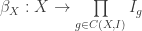 is defined by:
For each  ,
,  is the point
  such that
  for each (i.e. the
  coordinate of the point
  is
is  ).
).
For the proof that  is a homeomorphism, see A Beginning Look at Stone-Cech Compactification. We have the following definition.
Definition
Under the map ,  is the topological copy of within the cube
  . The Stone-Cech compactification of is defined to be the closure of in the cube , i.e., set
  .
.
When there is no ambiguity as to what the space is, the embedding is written as and the compactification  is written as (as in Figure 1 above). When more than one space is involved, we use subscripts to distinguish the embeddings, e.g., and
  .
.
_______________________________________________________________________________
Proof of Theorem U1
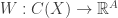
Let be a continuous function from into a compact Hausdorff space . Let be the Stone-Cech compactification of where is the homeomorphic embedding that defines . Since is a completely regular space, it has a Stone-Cech compactification  , where is the homeomorphic embedding. We also define a map
  from
from  into
into  . We have the following diagram.
Figure 2

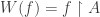
The desired function will be defined by 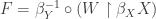 . The rest of the proof is to define and to show that this definition of makes sense.
To define the function , for each , let  such that
  (i.e. the
  coordinate of is the
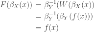
  coordinate of ). With the definition of , the diagram in Figure 2 commutes, i.e.,
Starting with a point (the upper left corner of the diagram), we can reach the same point in the lower right corner regardless the path we take ( or
or  ). The following shows the derivation.
_________________________________
It is straightforward to verify that the map is continuous. Based on  above, note that
  . The following derivation shows that
  .
.
With the above derivation, we now know that the function maps points of to points of  . So it makes sense to define . Note that for each , we have:
Then we have  and is the desired function.
_______________________________________________________________________________
Compactifications
In order to prove Theorem U1, we first have a basic discussion on compactifications. Most importantly, we pin down what we mean when we say two compactifications of are equivalent. In the process, we produce another characterization of Stone-Cech compactification (see Theorem C2 and Theorem U2 below).
Let be a completely regular space. A pair  is said to be a compactification of the space if
  is a compact Hausdorff space and
  is a homeomorphism from into such that
  is dense in . More informally, a compactification of the space can also be thought of as a compact space containing a topological copy of the space as a dense subspace.
Given a compactification , we use the notation  rather than the pair . By saying that is a compactification of , we mean is the compact space where
  is the homeomorphism embedding onto .
The Stone-Cech compactification construction above is an example of a compactification. There can be more than one compactification of a given space . For example, for  , we have the Stone-Cech compactification
  , which is a subspace of the cube
  . The circle
  contains a copy of the real line
  as a dense subspace, as does the unit interval
 ![[0,1]](https://s0.wp.com/latex.php?latex=%5B0%2C1%5D&bg=ffffff&fg=333333&s=0&c=20201002) . Thus both
. Thus both  and are also compactifications of . See A Beginning Look at Stone-Cech Compactification for a discussion of these examples.
We say that compactifications  and
and  are equivalent (we write
  ) if there exists a homeomorphism
 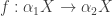 such that
  . In other words, the following diagram commutes.
Figure 3

Essentially, two compactifications and of are equivalent if there is a homeomorphism between the two and if each is mapped by to itself, i.e.,  is mapped to
  .
.
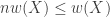
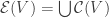
For a given completely regular space , let  be the class of all compactifications of . We define a partial order
  on . For and , both in , we say that
  if there is a continuous function
  such that
  . See Figure 4 below.
Figure 4

The following theorem ties the partial order to the equivalence relation  for compactifications.
Theorem 1
Let and be two compactifications of . Then  and if and only if .
Proof of Theorem 1
 With , there exists continuous
  such that
With , there exists continuous 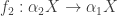 such that
Applying  to
to  , we have
 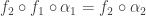 . Applying
  to this result, we have
Note that  is a map from into . The equation
  indicates that when is restricted to
  , it is the identity map. Thus agrees with the identity map on the dense set . This implies that must agree with the identity map on all of .
Likewise we can see that  must equal to the identity map on . So is a homeomorphism and it follows that and are equivalent compactifications of .
 This direction is straightforward. Let a homeomorphism that makes and equivalent (as described by Figure 3). Then the map implies and the map
  implies .
_______________________________________________________________________________
Another Characterization of the Stone-Cech Compactification
The next theorem says that the Stone-Cech compactification is the maximal compactification with respect to the partial order defined here. Furthermore, this property is unique (there is only one maximal compactification up to equivalence). This result will simplify the work when we need to show that a given compactification is equivalent to .
Theorem U2
The property in Theorem C2 is unique to . That is, if, among all compactifications of the space , is maximal with respect to the partial order , then  .
.
Proof Theorem C2
Let be any compactification of . Consider the continuous map  . By Theorem C1, can be extended to . In other words, there exists a continuous
 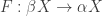 such that
  . The existence of the map implies that
  .
.
Proof Theorem U2
Let be another maximal compactification of . This implies that  . By Theorem C2, we have . By Theorem 1, must be equivalent to .
_______________________________________________________________________________
Proof of Theorem U1
We are now ready to prove Theorem U1.
Proof of Theorem U1
Let be a compactification of that satisfies the extension property in Theorem C1. In light of Theorem C2, we have . So we only need to show . Consider the map  . By the assumption that satisfies the extension property in Theorem C1, there exists a continuous function
 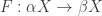 such that
  . The existence of implies that . By Theorem 1, must be equivalent to .
_______________________________________________________________________________
Blog Posts on Stone-Cech Compactification
_______________________________________________________________________________
Reference
- Engelking, R., General Topology, Revised and Completed edition, Heldermann Verlag, Berlin, 1989.
- Willard, S., General Topology, Addison-Wesley Publishing Company, 1970.
_______________________________________________________________________________


.
.
.
.
.
.


 be the set of all continuous functions
  . Then
  .
.
 be a space and let
  .
.


 -embedded in its Stone-Cech compactification
  . The subspace
  is extendable to a continuous
  .
. . Then
  illustrates that the
  can be regarded as
  where
where  is some closed and bounded interval. The
  such that
  .
. , let
, let  be the projection map from this cube into
  . Thus by assumption, each
  . Now define
 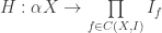 by the following:
 ,
,  such that
 , we have
  . Note that
  agrees with
  where
where 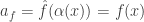 for each
  where
where  for each
 is continuous. Note that
  is dense in
  . Thus we have:
 together, we have the following:
 can be extended to
  where
where  be the first uncountable ordinal. Let
  be the successor ordinal of
  and
and  as topological spaces with the order topology derived from the well ordering of the ordinals. The space
  ,
,  (see result B in
  .
.


 or as a sequence
  such that each term (or coordinate)
 ![t_f \in I=[0,1]](https://s0.wp.com/latex.php?latex=t_f+%5Cin+I%3D%5B0%2C1%5D&bg=ffffff&fg=333333&s=0&c=20201002) .
. is the point in the cube such that for each
  . This map
 ![\Phi(x):\mathbb{R} \rightarrow [0,1]](https://s0.wp.com/latex.php?latex=%5CPhi%28x%29%3A%5Cmathbb%7BR%7D+%5Crightarrow+%5B0%2C1%5D&bg=ffffff&fg=333333&s=0&c=20201002) defined by:
defined by: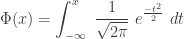
 is the cumulative distribution function (CDF) of the standard normal distribution. The following figure is the graph.
 and
and  , we cannot extend the function
  to a continuous function defined on
  defined on the open interval
  , which is a topological copy of
  to a continuous function defined on
  .
. , which maps
 ![[-1,1]](https://s0.wp.com/latex.php?latex=%5B-1%2C1%5D&bg=ffffff&fg=333333&s=0&c=20201002) . Based on Theorem C1,
. Based on Theorem C1,  can be extended to a function
 ![G: \beta \mathbb{R} \rightarrow [-1,1]](https://s0.wp.com/latex.php?latex=G%3A+%5Cbeta+%5Cmathbb%7BR%7D+%5Crightarrow+%5B-1%2C1%5D&bg=ffffff&fg=333333&s=0&c=20201002) .
. ![t \in [-1,1]](https://s0.wp.com/latex.php?latex=t+%5Cin+%5B-1%2C1%5D&bg=ffffff&fg=333333&s=0&c=20201002) , let
, let  . For example,
  is the set
  . Furthermore, for each
  , which is a compact set in
  for each
  is a discrete set in
  for each
  show that at minimum we are adding continuum many points to form
  ,
,  and
and  are disjoint (they are separated by disjoint open sets in
  ).
). , where
  where the topology is generated by a base consisting the half open intervals of the form
  . The Sorgenfrey plane is the square
  .
.  of open covers of
  satisfying the condition that for any open set
  ,
,  . When
  increases. In fact, this is how a development is defined for a metric space, where
  . Thus metric spaces are developable. There are plenty of non-metrizable Moore space. One example is the
  -set. Thus if a Moore space is normal, it is perfectly normal. Any Moore space has a
  is a
is a  ). It is a well known theorem that every compact space with a
  . Then
  is a countable base for
  -locally finite base for
  -space and for every discrete collection
  of closed sets in
  of open subsets of
  . For a proof of Bing’s metrization theorem, see page 329 of [1].
 such that
  . For each real number
  , define
  to be the set
  , define
  to be the set
  , and define
  . The topology on
  where
where  is isolated.
 , a basic open set is of the form
  where
where  and
and  .
. and
and  .
.![f:S \rightarrow [0,1]](https://s0.wp.com/latex.php?latex=f%3AS+%5Crightarrow+%5B0%2C1%5D&bg=ffffff&fg=333333&s=0&c=20201002) such that
such that  for all
  and
and  for all
  (using Urysohn lemma). But this function is not possible. It can be shown that any continuous function
 ![g:S \rightarrow [0,1]](https://s0.wp.com/latex.php?latex=g%3AS+%5Crightarrow+%5B0%2C1%5D&bg=ffffff&fg=333333&s=0&c=20201002) that maps
that maps  , the product of
  , is a space that has ccc but is not separable.
 be a collection of spaces where
  . Fix a point
  in the product. The sigma-product about the point
  and is the following subspace of the product space
 be separable. The product space
  for each
  for all
  is a ccc space that is not separable. Of course,
  in this case is the set of all
  such that
  for at most countably many
  is an example of a separable but not hereditarily separable space. Another interesting point is that
  of open subsets of
  (where
  ) is an uncountable disjoint collection of open subsets of
  of open subsets of
  , there is some
  , open subset of
  . Let
. Let  be the collection of all
  is a family of spaces such that
  has countable chain condition for every finite
  . Then
  has countable chain condition.
 , then
  and
and  are clear.
 such that
  for at most countably many
  . Let
. Let  be the collection of all
  (over all
  , a chain from
 ,
,  , and for
  ,
,  . For each
  , let
, let  be the following:
 . For
. For  , if
, if  ,
,  , and as a result
  . Thus the collection of all distinct
  is a collection of disjoint open sets in
  is traced back to at most countably many sets in open sets
  is a countable dense set in the space
  is a countable dense set in the product space
  . It follows that the product of finitely many separable spaces is separable. When the number of factors is infinite, the cardinality of the continuum is the dividing line. The product of separable spaces is sometimes separable (when the number of factors is less than or equal to continuum) and is sometimes not separable (when the number of factors is greater than continuum). For a discussion of this result, see
  of sets is said to be a Delta-system (or
  -system) if there is a set
  such that for every
  with
with  , we have
  . When such set
  of finite sets, there is an uncountable
  such that
  is a space that has ccc but is not separable.
 where
where  for all but finitely many
  . Let
. Let  , let
, let  be the finite set such that
  , and such that
  if and only if
  . Let
. Let  , then for any
  and
and  where
where  and
and  , we have
  , which leads to
  . Thus
  .
.  be the collection of all
  such that
  . For each
 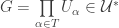 , let
, let  (i.e.
(i.e.  be the collection of all
  where
where  .
.  with
with  implies
  and
and  implies
  .
.  , which has ccc by hypothesis. So there exists
  with
with  . The above observation allows us to define a point
  , contradicting the assumption that
 space and for each
  , there is a continuous function
 ![f:X \rightarrow [0,1]](https://s0.wp.com/latex.php?latex=f%3AX+%5Crightarrow+%5B0%2C1%5D&bg=ffffff&fg=333333&s=0&c=20201002) such that
such that  and
and  . Note that the
  and
and  . So in a space that is not completely regular, there exist a closed set
  such that every real-valued continuous function
  is no longer completely regular. Let
  . The underlying set is
 where
where  .
. and at
 ")


![H_n=\left\{(x,0): n \le x \le n+1 \right\}=[n,n+1] \times \left\{0 \right\}](https://s0.wp.com/latex.php?latex=H_n%3D%5Cleft%5C%7B%28x%2C0%29%3A+n+%5Cle+x+%5Cle+n%2B1+%5Cright%5C%7D%3D%5Bn%2Cn%2B1%5D+%5Ctimes+%5Cleft%5C%7B0+%5Cright%5C%7D&bg=ffffff&fg=333333&s=0&c=20201002) . Let
. Let  be the x-axis.
  be a continuous function such that
  for infinitely many points
  , then for each integer
  where
where  ,
,  .
. . If
. If  is continuous and
  , then
  for all but countably many points
  .
. , then
  and the fact that
  be a subset of
  such that
 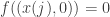 for all
  , let
, let  (the projection into the x-axis).
 for all but countably many
  . For each
  , let
, let  be a countably infinite subset of
  such that
  for all
  . The sets
  be the set of all
  where
where  . Consider
 ![J=[n+1,n+2] - \bigcup_{j \ge 1} B_j](https://s0.wp.com/latex.php?latex=J%3D%5Bn%2B1%2Cn%2B2%5D+-+%5Cbigcup_%7Bj+%5Cge+1%7D+B_j&bg=ffffff&fg=333333&s=0&c=20201002) . Note that
. Note that  is the complement of a countable set. Let
  which is a co-countable subset of
  . For each
  ,
,  (these points
  are in
  ). Thus by Claim 2, for each
  for infinitely many
  , we can continue the same argument to prove the same for the next interval
  . Continue the same inductive process, we can show that for each integer
  ,
,  .
.
![H_0=[0,1] \times \left\{0 \right\}](https://s0.wp.com/latex.php?latex=H_0%3D%5B0%2C1%5D+%5Ctimes+%5Cleft%5C%7B0+%5Cright%5C%7D&bg=ffffff&fg=333333&s=0&c=20201002) , which is a closed set in
, which is a closed set in  be continuous such that
  . Then we show that
  . This follows from the main result. By the main result derived above, for each integer
 ![w \in H_j =[j,j+1] \times \left\{0 \right\}](https://s0.wp.com/latex.php?latex=w+%5Cin+H_j+%3D%5Bj%2Cj%2B1%5D+%5Ctimes+%5Cleft%5C%7B0+%5Cright%5C%7D&bg=ffffff&fg=333333&s=0&c=20201002) . Then
. Then  has no choice by to be zero as well.
 , the closure is
  . Furthermore,
  . For each closed set
  with
with  , choose some integer
  . Then we have
  . This establishes the regularity of
  be the set of all
  and
and  be the set of all
 ![\rho: S \rightarrow [0,1]](https://s0.wp.com/latex.php?latex=%5Crho%3A+S+%5Crightarrow+%5B0%2C1%5D&bg=ffffff&fg=333333&s=0&c=20201002) such that
such that  and
and  .
.  is not possible. To see this, suppose
  for infinitely many
  , namely all
  where
where  . But
. But  for all irrational