Drawing more Sorgenfrey continuous functions

Posted on January 1, 2018 by Dan Ma

In this previous post, we draw continuous functions on the Sorgenfrey line $S$ to gain insight about the function $C_p(S)$ . In this post, we draw more continuous functions with the goal of connecting $C_p(S)$ and $C_p(D)$ where $D$ is the double arrow space. For example, $C_p(D)$ can be embedded as a subspace of $C_p(S)$ . More interestingly, both function spaces $C_p(D)$ and $C_p(S)$ share the same closed and discrete subspace of cardinality continuum. As a result, the function space $C_p(D)$ is not normal.

Double Arrow Space

The underlying set for the double arrow space is $D=[0,1] \times \{ 0,1 \}$ , which is a subset in the Euclidean plane.

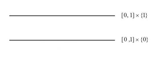
Figure 1 – The Double Arrow Space

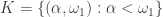
The name of double arrow comes from the fact that an open neighborhood of a point in the upper line segment points to the right while an open neighborhood of a point in the lower line segment points to the left. This is demonstrated in the following diagram.

Figure 2 – Open Neighborhoods in the Double Arrow Space

More specifically, for any $a$ with $0 \le a < 1$ , a basic open set containing the point $(a,1)$ is of the form $\displaystyle \biggl[ [a,b) \times \{ 1 \} \biggr] \cup \biggl[ (a,b) \times \{ 0 \} \biggr]$ , painted red in Figure 2. One the other hand, for any $a$ with $0<a \le 1$ , a basic open set containing the point $(a,0)$ is of the form $\biggl[ (c,a) \times \{ 1 \} \biggr] \cup \biggl[ (c,a] \times \{ 0 \} \biggr]$ , painted blue in Figure 2. The upper right point $(1,1)$ and the lower left point $(0,0)$ are made isolated points.

The double arrow space is a compact space that is perfectly normal and not metrizable. Basic properties of this space, along with those of the lexicographical ordered space, are discussed in this previous post.

The drawing of continuous functions in this post aims to show the following results.

The function space $C_p(D)$ can be embedded as a subspace in the function $C_p(S)$ .
Both function spaces $C_p(D)$ and $C_p(S)$ share the same closed and discrete subspace of cardinality continuum.
The function space $C_p(D)$ is not normal.

Drawing a Map from Sorgenfrey Line onto Double Arrow Space

In order to show that $C_p(D)$ can be embedded into $C_p(S)$ , we draw a continuous map from the Sorgenfrey line $S$ onto the double arrow space $D$ . The following diagram gives the essential idea of the mapping we need.

Figure 3 – Mapping Sorgenfrey Line onto Double Arrow Space

The mapping shown in Figure 3 is to map the interval $[0,1]$ onto the upper line segment of the double arrow space, as demonstrated by the red arrow. Thus $x \mapsto (x,1)$ for any $x$ with $0 \le x \le 1$ . Essentially on the interval $[0,1]$ , the mapping is the identity map.

On the other hand, the mapping is to map the interval $[-1,0)$ onto the lower line segment of the double arrow space less the point $(0, 0)$ , as demonstrated by the blue arrow in Figure 3. Thus $-x \mapsto (x,0)$ for any $-x$ with $0<x \le 1$ . Essentially on the interval $[-1,0)$ , the mapping is the identity map times -1.

The mapping described by Figure 3 only covers the interval $[-1,1]$ in the domain. To complete the mapping, let $x \mapsto (1,1)$ for any $x \in (1, \infty)$ and $x \mapsto (0,0)$ for any $x \in (-\infty, -1)$ .

Let $h$ be the mapping that has been described. It maps the Sorgenfrey line onto the double arrow space. It is straightforward to verify that the map $h: S \rightarrow D$ is continuous.

Embedding

We use the following fact to show that $C_p(D)$ can be embedded into $C_p(S)$ .

Suppose that the space $Y$ is a continuous image of the space $X$ . Then $C_p(Y)$ can be embedded into $C_p(X)$ .

Based on this result, $C_p(D)$ can be embedded into $C_p(S)$ . The embedding that makes this true is $E(f)=f \circ h$ for each $f \in C_p(D)$ . Thus each function $f$ in $C_p(D)$ is identified with the composition $f \circ h$ where $h$ is the map defined in Figure 3. The fact that $E(f)$ is an embedding is shown in this previous post (see Theorem 1).

Same Closed and Discrete Subspace in Both Function Spaces

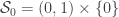
The following diagram describes a closed and discrete subspace of $C_p(S)$ .

Figure 4 – a family of Sorgenfrey continuous functions

For each $0<a<1$ , let $f_a: S \rightarrow \{0,1 \}$ be the continuous function described in Figure 4. The previous post shows that the set 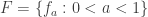$F=\{ f_a: 0<a<1 \}$ is a closed and discrete subspace of $C_p(S)$ . We claim that $F \subset C_p(D) \subset C_p(S)$ .

To see that $F \subset C_p(D)$ , we define continuous functions 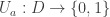$U_a: D \rightarrow \{0,1 \}$ such that $f_a=U_a \circ h$ . We can actually back out the map $U_a$ from $f_a$ in Figure 4 and the mapping $h$ . Here’s how. The function $f_a$ is piecewise constant (0 or 1). Let’s focus on the interval $[-1,1]$ in the domain of $f_a$ .

Consider where the function $f_a$ maps to the value 1. There are two intervals, $[a,1)$ and $[-1,-a)$ , where $f_a$ maps to 1. The mapping $h$ maps $[a,1)$ to the set $[a,1) \times \{ 1 \}$ . So the function $U_a$ must map $[a,1) \times \{ 1 \}$ to the value 1. The mapping $h$ maps $[-1,-a)$ to the set $(a,1] \times \{ 0 \}$ . So $U_a$ must map $(a,1] \times \{ 0 \}$ to the value 1.

Now consider where the function $f_a$ maps to the value 0. There are two intervals, $[0,a)$ and $[-a,0)$ , where $f_a$ maps to 0. The mapping $h$ maps $[0,a)$ to the set $[0,a) \times \{ 1 \}$ . So the function $U_a$ must map $[0,a) \times \{ 1 \}$ to the value 0. The mapping $h$ maps $[-a,0)$ to the set $(0,a] \times \{ 0 \}$ . So $U_a$ must map $(0,a] \times \{ 0 \}$ to the value 0.

To take care of the two isolated points $(1,1)$ and $(0,0)$ of the double arrow space, make sure that $U_a$ maps these two points to the value 0. The following is a precise definition of the function $U_a$ .

$\displaystyle U_a(y) = \left\{ \begin{array}{ll} \displaystyle 1 &\ \ \ \ \ \ y \in [a,1) \times \{ 1 \} \\ \text{ } & \text{ } \\ \displaystyle 1 &\ \ \ \ \ \ y \in (a,1] \times \{ 0 \} \\ \text{ } & \text{ } \\ 0 &\ \ \ \ \ \ y \in (0,a] \times \{ 0 \} \\ \text{ } & \text{ } \\ 0 &\ \ \ \ \ \ y \in [0,a) \times \{ 1 \} \\ \text{ } & \text{ } \\ 0 &\ \ \ \ \ \ y=(0,0) \text{ or } y = (1,1) \end{array} \right.$

The resulting $U_a$ is a translation of $f_a$ . Under the embedding $E$ defined earlier, we see that $E(U_a)=f_a$ . Let $U=\{ U_a: 0<a<1 \}$ . The set $U$ in $C_p(D)$ is homeomorphic to the set $F$ in $C_p(S)$ . Thus $U$ is a closed and discrete subspace of $C_p(D)$ since $F$ is a closed and discrete subspace of $C_p(S)$ .

Remarks

The drawings and the embedding discussed here and in the previous post establish that $C_p(D)$ , the space of continuous functions on the double arrow space, contains a closed and discrete subspace of cardinality continuum. It follows that $C_p(D)$ is not normal. This is due to the fact that if $C_p(X)$ is normal, then $C_p(X)$ must have countable extent (i.e. all closed and discrete subspaces must be countable).

While $C_p(D)$ is embedded in $C_p(S)$ , the function space $C_p(S)$ is not embedded in $C_p(D)$ . Because the double arrow space is compact, $C_p(D)$ has countable tightness. If $C_p(S)$ were to be embedded in $C_p(D)$ , then $C_p(S)$ would be countably tight too. However, $C_p(S)$ is not countably tight due to the fact that $S \times S$ is not Lindelof (see Theorem 1 in this previous post).

Reference

Arkhangelskii, A. V., Topological Function Spaces, Mathematics and Its Applications Series, Kluwer Academic Publishers, Dordrecht, 1992.
Tkachuk V. V., A $C_p$ -Theory Problem Book, Topological and Function Spaces, Springer, New York, 2011.

$\text{ }$

Dan Ma math

Daniel Ma mathematics

$\copyright$ 2018 – Dan Ma

Normal x Compact Needs Not be Normal

Posted on October 19, 2009 by Dan Ma

This is to present a non-normal cross product where one factor is a normal space and the other factor is a compact space. The normal space is $X=[0,\omega_1)$ and the compact space is $Y=[0,\omega_1]$ . I would like to show that $X \times Y$ is not normal. For a basic discussion on these ordinal spaces with the order topology, see this previous post.

In addition to demonstrating an example meeting the criteria set forth in the title, I would like to look at this through two angles. Because these spaces have the ordered topology, they are hereditarily normal (completely normal). Note that $X \times Y$ is a subspace of $Y \times Y$ . Thus $Y \times Y$ fails to be hereditarily normal, demonstrating that hereditarily normal x hereditarily normal needs not be hereditarily normal. Another example of this is the double arrow space. In this previous post, I showed that the square of the double arrow space is not hereditarily normal. The double arrow space is perfectly normal and is thus a stronger example in this regard since it shows the square of a perfectly normal space needs not be hereditarily normal. But the uncountable ordinal spaces of $[0,\omega_1)$ and $[0,\omega_1]$ are important counterexamples as well as building blocks for other counterexamples. So for the record, I present them here.

For the second angle, these two spaces show that hereditarily normality is not “nice” enough to prevent non-normal product.

In proving $X \times Y$ is not normal, the Pressing Down Lemma is used. A subset $S$ of $X=[0,\omega_1)$ is a stationary set if $S$ meets every closed and unbounded set in $X$ . The following is one version of the Pressing Down Lemma (see Lemma 6.15 on p. 80 of [1] for a more general version).

Pressing Down Lemma

$S$

$[0,\omega_1)$

$f:S \rightarrow \omega_1$

$\gamma \in S$

$f(\gamma)<\gamma$

$\alpha<\omega_1$

$f^{-1}\lbrace{\alpha}\rbrace$

$[0,\omega_1)$

To show that $X \times Y$ is not normal, let $H$ and $K$ be the following sets.

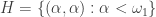
$H=\lbrace{(\alpha,\alpha):\alpha<\omega_1}\rbrace$

$K=\lbrace{(\alpha,\omega_1):\alpha<\omega_1}\rbrace$

These two sets are disjoint and closed in $X \times Y$ . Let $U$ and $V$ be open such that $H \subset U$ and $K \subset V$ . It follows that $U \cap V \neq \phi$ .

For each $\alpha<\omega_1$ , let $g(\alpha)<\omega_1$ such that $[g(\alpha),\alpha] \times [g(\alpha),\alpha] \subset U$ . Since $g$ is a pressing down function, there is some $\delta<\omega_1$ and there is a stationary set $S$ such that all points in $S$ are mapped to $\delta$ by $g$ . Specifically, for each $\alpha \in S$ , we have:

$[\delta,\alpha] \times [\delta,\alpha] \subset U$

Choose $\beta_0>\delta$ and let $\beta=\beta_0+1$ . We have $(\beta,\omega_1) \in K \subset V$ . Choose $\gamma>\delta$ such that

$\lbrace{\beta}\rbrace \times [\gamma,\omega_1] \subset V$

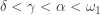Choose $\alpha \in S$ such that $\delta < \beta<\alpha$ and $\delta<\gamma<\alpha<\omega_1$ . We have the following set inclusions:

$\lbrace{\beta}\rbrace \times [\gamma,\alpha] \subset [\delta,\alpha] \times [\delta,\alpha] \subset U$

$\lbrace{\beta}\rbrace \times [\gamma,\alpha] \subset \lbrace{\beta}\rbrace \times [\gamma,\omega_1] \subset V$

Thus $U \cap V \neq \phi$ . This completes the proof that the product $X \times Y$ is not normal.

____________________________________________________________________

Reference

Kunen, K., Set Theory, An Introduction to Independence Proofs, North-Holland, Amsterdam, 1980.

____________________________________________________________________

Revised February 3, 2014.
$\copyright \ 2014 \text{ by Dan Ma}$

The Lexicographic Order and The Double Arrow Space

Posted on October 7, 2009 by Dan Ma

This post is a basic discussion on the unit square with the lexicographic order and one of its subspace called the double arrow space. The goal is to establish several basic facts of these two spaces. Both of these spaces are compact non-metrizable spaces. The double arrow space consists of the top and bottom edges of the unit square. The double arrow has a strong connection to the Sorgenfrey Line and its square is an example of a space that is normal that is not completely normal. The unit square with the lexicographic order is an example of a completely normal space that is not perfectly normal.

____________________________________________________________________

Defining the spaces

Let $I$ be the unit interval $[0,1]$ . Let $\mathcal{X}$ be $I\times I$ . Consider the lexicographic order on $\mathcal{X}$ . This is the linear order $<$ defined by letting $(a,b)<(c,d)$ whenever $a<c$ or $(a=c$ and $b<d)$ . The goal is to consider the square with the topology induced by this linear order. For $p=(a,b)$ and $q=(c,d)$ , $<p,q>$ is the notation in this post for open intervals in the unit square.

To facilitate further discussion, let’s look at the following subsets of $\mathcal{X}$ .

$\mathcal{A}_0=I \times \lbrace{0}\rbrace$

$\mathcal{A}_1=I \times \lbrace{1}\rbrace$

$\mathcal{B}_0=\lbrace{0}\rbrace \times I$

$\mathcal{B}_1=\lbrace{1}\rbrace \times I$

$\mathcal{S}_0=(0,1) \times \lbrace{0}\rbrace$

$\mathcal{S}_1=(0,1) \times \lbrace{1}\rbrace$

$\mathcal{A}=\mathcal{A}_0 \cup \mathcal{A}_1$

The subspace $\mathcal{A}$ is called the double arrow space. In this post, my aim is to establish some basic facts about the double arrow space $\mathcal{A}$ and then the unit square $\mathcal{X}$ .

Double arrow space

$\mathcal{A}$

$\mathcal{A}^2$

Unit square with lexicographic order

$\mathcal{X}$

____________________________________________________________________

Open intervals in these spaces

Before proving the results stated above, let’s make sense of the open intervals in $\mathcal{X}$ and then in $\mathcal{A}$ . The open intervals for points in $\mathcal{X}-\mathcal{A}$ are essentially the usual open intervals. For example, for the point $(0.5,0.5)$ , the following is an open interval in $\mathcal{X}$ .

$\lbrace{0.5}\rbrace \times (0.25,0.75)$

Because of this, $\mathcal{X}$ has an uncountable collection of pairwise disjoint open intervals (thus does not have ccc and is not separable). Also, a vertical line in $\mathcal{X}$ of the form $\lbrace{t}\rbrace \times I$ is a homeomorphic copy of the unit interval $[0,1]$ with the usual topology.

The more interesting open neighborhoods are for the points in the top and bottom lines (i.e. the double arrow space). Let’s look an example of an open interval in $\mathcal{X}$ for the point $(0.5,1)$ . Consider the open interval $<p,q>$ where $p=(0.5,0.9)$ and $q=(0.6,0.2)$ . It follows that the open interval $<p,q>=L \cup M \cup R$ where

$L=\lbrace{0.5}\rbrace \times (0.9,1]$

$M=(0.5,0.6) \times I$

$R=\lbrace{0.6}\rbrace \times [0,0.2)$

Note that $M$ is the vertical strip in the middle, $L$ is the left edge, and $R$ is the right edge. If you look at $<p,q>\cap{\mathcal{A}}$ , then the open interval for the point $(0.5,1)$ becomes

$\biggl((0.5,0.6] \times \lbrace{0}\rbrace \biggr) \cup \biggl( [0.5,0.6) \times \lbrace{1}\rbrace \biggr)$

The above is also an open interval in $\mathcal{A}$ containing the point $(0.6,0)$ . Similarly, an example of an open interval containing the point $(0.5,0)$ is:

$\biggl( (0.4,0.5] \times \lbrace{0}\rbrace \biggr) \cup \biggl([0.4,0.5) \times \lbrace{1}\rbrace\biggr)$

Based on the above examples of open intervals, open intervals in $\mathcal{A}$ have the following form, hence the term “double arrow”.

$\biggl((a,b] \times \lbrace{0}\rbrace\biggr) \cup \biggl([a,b) \times \lbrace{1}\rbrace\biggr)$

____________________________________________________________________

Proofs

The double arrow space contains two copies of the Sorgenfrey line. So knowing the basic properties of the Sorgenfrey line will help follow the proofs of A through D below. Information about the Sorgenfrey line can be found in the following blog post.

A Note On The Sorgenfrey Line

A Short Note About The Sorgenfrey Line

Proof of A. I now proof that the double arrow space $\mathcal{A}$ is compact. I do so by showing that it is Lindelof and countably compact. A space is countably compact if any countable open cover has a finite subcover (equivalently, any infinite subspace has a limit point). Here, limit point is in the topological sense (i.e. the point $p$ is a limit point of the set $K$ if any open set containing $p$ contains a point of $K$ different from $p$ ).

Note that $\mathcal{S}_0$ and $\mathcal{S}_1$ as defined above are homeomorphic copies of the Sorgenfrey Line. Thus $\mathcal{A}$ is made of of two copies of the Sorgenfrey Line plus 4 points. This shows that $\mathcal{A}$ is hereditarily Lindelof.

Pick an infinite subset $W$ of $\mathcal{A}$ . Then either the top or the bottom contains infinitely many points of $W$ . Assume the top does. There is a point $(q,1)$ that is a limit point of $W \cap \mathcal{A}_1$ in the usual topology. If the point $(q,1)$ is a right-sided limit point of $W \cap \mathcal{A}_1$ in the usual topology, then the point $(q,1)$ is a limit point of $W$ in the order topology. If the point $(q,1)$ is a left-sided limit point of $W \cap \mathcal{A}_1$ in the usual topology, then the point $(q,0)$ is a limit point of $W$ in the order topology.

Proof of B, C and D. As observed in the proof of A, the double arrow space is the union of 2 copies of the Sorgenfrey Line plus 4 points. Thus it is hereditarily Lindelof, hereditarily separable and perfectly normal.

Note that $\mathcal{A}^2$ contains a copy of the Sorgenfrey Plane. Thus it is not hereditarily normal. This also implies that both the double arrow space and the unit square with the lexicographic order are not metrizable.

Proof of E. Let $\mathcal{U}$ be an open cover for $\mathcal{X}$ that consists of open intervals. Since $\mathcal{A}$ is compact, there exists a finite collection of open intervals $\lbrace{U_0,U_1,...,U_n}\rbrace$ from $\mathcal{U}$ that cover $\mathcal{A}$ . Based on the above observation about open intervals of points in the double arrow space, the open intervals $U_i$ cover all the points in $\mathcal{X}-\mathcal{A}$ except possibly the left and right edges of the open intervals $U_i$ . With the topology inherited from the order topology, each of the edges is homeomorphic to the unit interval with the usual topology. Thus there are finitely many open intervals from $\mathcal{U}$ that cover these left and right edges. Thus $\mathcal{U}$ has a finite subcover and $\mathcal{X}$ is compact.

Proof of F, G, H. These are clear based on the above observation made about the open intervals in the unit square.

Proof of I. I show here that $\mathcal{A}$ cannot be a $G_\delta$ set in the unit square $\mathcal{X}$ . For each $n<\omega$ , let $U_n$ be an open set in $\mathcal{X}$ such that $\mathcal{A} \subset U_n$ . Since $\mathcal{A}$ is compact, we can assume that $U_n$ is the union of finitely many open intervals. Based on the observation given above, each $U_n$ covers all of $\mathcal{X}-\mathcal{A}$ except for finitely many vertical lines (the left and right edges of these open intervals). Pick one vertical line that is not one of the vertical edges from the open intervals $U_n$ . Clearly this vertical line is covered by $U_n$ for each $n<\omega$ . Thus $\mathcal{A}$ is not a $G_\delta$ set in $\mathcal{X}$ .

Comment. The double arrow space is made up of 2 copies of the Sorgenfrey Line and the 4 corner points. It follows that it is hereditarily Lindelof and perfectly normal. However, since the square of the double arrow space contains a copy of the Sorgenfrey Plane, the square of the double arrow space is not hereditarily normal, thus showing that normality is not a hereditary notion. The square of the double arrow space $\mathcal{A}^2$ is a handy example of a normal space that is not completely normal. This implies both the double arrow space and the unit square with the lexicographic order not metrizable. The space $\mathcal{A}^2$ also demonstrates that hereditarily normality is not preserved by Cartesian product.

The unit square with the lexicographic order topology is completely normal ([Steen & Seebach]). Thus it is an example of a space that completely normal (T4) but not perfectly normal (T5).

Reference

Counterexamples In Topology

Dan Ma's Topology Blog

Expository Articles In General Topology

Tag Archives: Double arrow space

Drawing more Sorgenfrey continuous functions

Normal x Compact Needs Not be Normal

The Lexicographic Order and The Double Arrow Space