Let  be a completely regular space. Let
  be the Stone-Cech compactification of . We present two characterizations of in addition to three others that are discussed previously. In all, these five characterizations can help us derive many of the basic properties of . We prove the following theorems.
Theorem C4
Let be a completely regular space. Every two completely separated subsets of have disjoint closures in .
Theorem U4
The property described in Theorem C4 is unique to . That is, if  is a compactification of satisfying the condition that every two completely separated subsets of have disjoint closures in , then must be .
Theorem C5
Let be a normal space. Then every two disjoint closed subsets of have disjoint closures in .
Theorem U5
If is a compactification of satisfying the property that every two disjoint closed subsets of have disjoint closures in , then is normal and must be .
The C theorem and U theorem with the same number work as a pair. The C theorem asserts that has a certain property. The corresponding U theorem asserts that of all the compactifications of , is the only one with the property in question. Whenever we can show a given compactification does not possess the property described in the C-U theorem pair, we know that that compactification is not (consequence of the C theorem). Whenever we can show that a given compactification has the property described in the C-U theorem pair, we know that that compactification must be (a consequence of the U theorem).
Three other sets of characterizations (Theorems C1, U1, C2, U2, C3 and U3) have been established previously. See the links found below.
___________________________________________________________________________________
Completely Separated Sets
Let  be a completely regular space. Let
  and
and  . The sets
  and
and  are said to be completely separated in if there is a continuous function
 ![f:Y \rightarrow [0,1]](https://s0.wp.com/latex.php?latex=f%3AY+%5Crightarrow+%5B0%2C1%5D&bg=ffffff&fg=333333&s=0&c=20201002) such that for each
such that for each  ,
,  and for each
  ,
,  (this can also be expressed as
  and
and  ). If and are completely separated,
  and
and  are necessarily disjoint closed sets, since
  and
and  .
.
The Urysohn’s lemma can be stated as: a space is a normal space if and only if every two disjoint closed sets are completely separated. Thus disjoint closed sets are not necessarily completely separated (such sets can be found in non-normal spaces).
___________________________________________________________________________________
Some Helpful Results
To prove Theorem U4, we need a lemma and a theorem. Most of the work in proving Theorem U4 is carried out in Theorem 2 below.
Lemma 1
Let be a compact space. Let  be an open subset of . Let
  be a collection of compact subsets of such that
  . Then there exists a finite collection
  such that
  .
.
Proof of Lemma 1
Let  , which is compact. Let
  be the collection of all
  where
where  . Note that implies that
  . Thus is a collection of open sets covering the compact set
  . We have
  such that
  . Each
  for some
  . Now
. Now  is the desired finite collection.
Theorem 2
Let  be a completely regular space. Let
  be a dense subspace of . Let
  be a continuous function from into a compact space . Suppose that every two completely separated subsets of have disjoint closures in . Then
  can be extended to a continuous
  .
.
Proof
For each  , let
, let  be the set of all open subsets of containing
  . For each , let
  be the set of all
  where
where  . Note that each consists of compact subsets of . The theorem is established by proving the following claims.
Claim 1
For each , the collection has non-empty intersection.
For any  , we have the following:
The above shows that has the finite intersection property (f. i. p.). It is a well known fact that in a compact space, any collection of sets with f. i. p. has non-empty intersection (see [1] or [2] or see The Finite Intersection Property in Compact Spaces and Countably Compact Spaces in this blog).
Claim 2
For each ,  has only one point.
Let . Suppose that
 where
where 
Then there exist open subsets  and
and  of such that
  ,
,  and
and  . Since is compact, it is a normal space. By the Urysohn’s lemma, there exists a continuous
 ![g:K \rightarrow [0,1]](https://s0.wp.com/latex.php?latex=g%3AK+%5Crightarrow+%5B0%2C1%5D&bg=ffffff&fg=333333&s=0&c=20201002) such that for each
such that for each  ,
,  and for each
  ,
,  . Then because of the function
 ![g \circ f:S \rightarrow [0,1]](https://s0.wp.com/latex.php?latex=g+%5Ccirc+f%3AS+%5Crightarrow+%5B0%2C1%5D&bg=ffffff&fg=333333&s=0&c=20201002) , the sets
, the sets  and
and  are completely separated sets in . By assumption, these two sets have disjoint closures in , i.e.,
The point cannot be in both of the sets in  . Assume the following:
Then  . Note that
  . Furthermore,
  . Thus we have:
Since  and is an open set containing
  , contains at least one point of
  . Choose
  such that
  . Now choose
  such that
  . First we have
  and thus
  . Secondly since
  , we have
  . We now have and
  , a contradiction. If we assume
  , we can also derive a contradiction in a similar derivation. Thus the assumption in
  above is faulty. The intersection can only have one point.
Claim 3
For each  ,
,  .
.
Let . Suppose that  where
where  . the rest of the proof for Claim 3 is similar to that of Claim 2. For the sake of completeness, we give a sketch.
There exist open subsets and of such that  ,
,  and . By the same argument as in Claim 2, we have the condition , i.e.,
  . Since
  ,
,  . The remainder of the proof of Claim 3 is the same as above starting with condition
  with
with  . A contradiction will be obtained. We can conclude that the assumption that where must be faulty. Thus Claim 3 is established.
Claim 4
For each , define by letting  be the point in . Note that this function extends . Furthermore, the map is continuous.
To show  is continuous, let and let
  where
where  is open in . The collection is a collection of compact subsets of such that
  . By Lemma 1, there exists
  such that
  . By the definition of , there exists
  such that each
  . Let
. Let  . We have:
Note that  is an open subset of and
  . We show that
  . Pick
  . According to the definition of
  , we have
  . Since
  , we have
  . Thus by
  , we have
  . Thus Claim 4 is established.
With all the above claims established, we completed the proof of Theorem 2.
___________________________________________________________________________________
Theorem C4 and Theorem U4
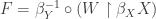
Proof of Theorem C4
In proving C4, we use Theorem C3, which is found in C*-Embedding Property and Stone-Cech Compactification.
Let and be two completely separated sets in . Then there exists some continuous ![g:X \rightarrow [0,1]](https://s0.wp.com/latex.php?latex=g%3AX+%5Crightarrow+%5B0%2C1%5D&bg=ffffff&fg=333333&s=0&c=20201002) such that for each
such that for each  ,
,  and for each
  ,
,  . By Theorem C3,
  is extended by some continuous
 ![G:\beta X \rightarrow [0,1]](https://s0.wp.com/latex.php?latex=G%3A%5Cbeta+X+%5Crightarrow+%5B0%2C1%5D&bg=ffffff&fg=333333&s=0&c=20201002) . The sets
. The sets  and
and  are disjoint closed sets in . Furthermore,
  and
and  . Thus and have disjoint closures in .
Proof of Theorem U4
In proving U4, we use Theorem U1, which is stated and proved in Two Characterizations of Stone-Cech Compactification.
Suppose that is a compactification of satisfying the condition that every two completely separated subsets of have disjoint closures in . Let  be a continuous function from into a compact space . By Theorem 2, can be extended by a continuous
  . By Theorem U1, must be .
___________________________________________________________________________________
Theorem C5 and Theorem U5
Proof of Theorem C5
Let be a normal space. According to the Urysohn’s lemma, every two disjoint closed sets are completely separated. Thus by Theorem C4, every two disjoint closed subsets of have disjoint closures in .
Proof of Theorem U5
Suppose that is a compactification of satisfying the property that every two disjoint closed subsets of have disjoint closures in . To show that is normal, let and be disjoint closed subsets of . By assumption about , and (closures in ) are disjoint. Since are compact and Hausdorff, is normal. Then and can be separated by disjoint open subsets and  of . Thus
  and
and  are disjoint open subsets of separating and .
We use Theorem U4 to prove Theorem U5. We show that satisfies Theorem U4. To this end, let and be two completely separated sets in . We show that and have disjoint closures in . There exists some continuous ![f:X \rightarrow [0,1]](https://s0.wp.com/latex.php?latex=f%3AX+%5Crightarrow+%5B0%2C1%5D&bg=ffffff&fg=333333&s=0&c=20201002) such that for each ,
such that for each ,  and for each ,
  . Then
  and
and  are disjoint closed sets in such that
  and
and  . By assumption about , and have disjoint closures in . This implies that and have disjoint closures in . Then by Theorem U4, must be .
___________________________________________________________________________________
Blog Posts on Stone-Cech Compactification
___________________________________________________________________________________
Reference
- Engelking, R., General Topology, Revised and Completed edition, Heldermann Verlag, Berlin, 1989.
- Willard, S., General Topology, Addison-Wesley Publishing Company, 1970.
___________________________________________________________________________________


![I=[0,1]](https://s0.wp.com/latex.php?latex=I%3D%5B0%2C1%5D&bg=ffffff&fg=333333&s=0&c=20201002)

is normal.
.


 , then there exists a free sequence
  .
.


![[0,\alpha] \times Y](https://s0.wp.com/latex.php?latex=%5B0%2C%5Calpha%5D+%5Ctimes+Y&bg=ffffff&fg=333333&s=0&c=20201002)


![O=(\theta,\omega_1] \times V](https://s0.wp.com/latex.php?latex=O%3D%28%5Ctheta%2C%5Comega_1%5D+%5Ctimes+V&bg=ffffff&fg=333333&s=0&c=20201002)


![(\delta,y_\delta) \in (\theta,\omega_1] \times V](https://s0.wp.com/latex.php?latex=%28%5Cdelta%2Cy_%5Cdelta%29+%5Cin+%28%5Ctheta%2C%5Comega_1%5D+%5Ctimes+V&bg=ffffff&fg=333333&s=0&c=20201002)


![[\alpha,\gamma] \times \left\{y \right\}](https://s0.wp.com/latex.php?latex=%5B%5Calpha%2C%5Cgamma%5D+%5Ctimes+%5Cleft%5C%7By+%5Cright%5C%7D&bg=ffffff&fg=333333&s=0&c=20201002)
![\theta \in [\alpha,\gamma]](https://s0.wp.com/latex.php?latex=%5Ctheta+%5Cin+%5B%5Calpha%2C%5Cgamma%5D&bg=ffffff&fg=333333&s=0&c=20201002)


 is paracompact.
 -compact, then
  of subsets of
  (in words every point of the space belongs to one set in the collection). Furthermore,
  be covers of the space
  , there is some
  such that
  , there is a non-empty open subset
  and
and  of subsets of the space
  such that each
  is a locally finite collection of subsets of
  of
of  such that
  for each
  -subsets.
 such that
  where each
  is a closed subset of
  , let
, let  be open in
  .
.  be the set of all
  . Let
. Let  be a locally finite refinement of
  . Let
. Let  be the following:
 is a
is a  such that
  , there is an open set
  such that
  .
. such that
  is a cover of
  . By the Tube Lemma, for each
  such that
  . Since
  be a locally finite open refinement of
  such that
  for each
  . We claim that
  is a locally finite open refinement of
  . Then
  for some
  and
and  . Thus,
  for some
  . Secondly, it is clear that
  . Then
  can meet only finitely many sets in
  , which is the Stone-Cech compactification of
  is paracompact. Note that
  and each
  is a closed subset of


 , the Stone-Cech compactification of the discrete space of the non-negative integers,
  . We use several characterizations of Stone-Cech compactification to find out what
  denote the cardinality of the real line
  . We prove the following facts.
 .
. is an isolated point.
 -point.
 be the set of all continuous functions from
 ![[0,1]^{C(X,I)}](https://s0.wp.com/latex.php?latex=%5B0%2C1%5D%5E%7BC%28X%2CI%29%7D&bg=ffffff&fg=333333&s=0&c=20201002) which is the closure of the image of
which is the closure of the image of ![\beta:X \rightarrow [0,1]^{C(X,I)}](https://s0.wp.com/latex.php?latex=%5Cbeta%3AX+%5Crightarrow+%5B0%2C1%5D%5E%7BC%28X%2CI%29%7D&bg=ffffff&fg=333333&s=0&c=20201002) (for the details, see
(for the details, see  be a continuous function from
  such that
  .
.
 .
.
 .
.
 -embedded in its Stone-Cech compactification
  can be extended to a continuous
  . Then
  where
where  is the density (the smallest cardinality of a dense set in
  being a countable space,
  .
.  . Consider the cube
  where
where  be a countable dense set. Let
  be a bijection. Clearly
  . Note that the image
  is dense in
  . Thus
  . Thus
  . The same function
  (see Lemma 2 in
 and
and  . By Theorem C3.1,
  and
and  . Thus
  .
.  . Define
 ![\gamma:X \rightarrow [0,1]](https://s0.wp.com/latex.php?latex=%5Cgamma%3AX+%5Crightarrow+%5B0%2C1%5D&bg=ffffff&fg=333333&s=0&c=20201002) by letting
by letting  for all
  and
and  for all
  . Since both
  is continuous. By Theorem C3,
 ![\Gamma:\beta X \rightarrow [0,1]](https://s0.wp.com/latex.php?latex=%5CGamma%3A%5Cbeta+X+%5Crightarrow+%5B0%2C1%5D&bg=ffffff&fg=333333&s=0&c=20201002) . Note that
. Note that  and
and  . Thus
  .
.  ,
,  (the closure of
  in
in  be a set that is both closed and open in
  where
where  .
.
 . Either
  or
or  . Thus
  . We claim that
  , it follows that
  . To show
  , pick
  . If
. If  , then
  . So focus on the case that
  . It is clear that
  where
where  . But every open set containing
  must contain some points of
  . Lemma 3 shows that
  . Lemma 4 shows that
  . Thus
  . We claim that
  with
with  . Let
. Let  with
with  . Let
. Let  .
.  . There exists open
  such that
  and
and  . Then
  , which is a contradiction. So we have
  . Thus
 ![g:A \rightarrow [0,1]](https://s0.wp.com/latex.php?latex=g%3AA+%5Crightarrow+%5B0%2C1%5D&bg=ffffff&fg=333333&s=0&c=20201002) be any function (necessarily continuous). Let
be any function (necessarily continuous). Let ![f:\omega \rightarrow [0,1]](https://s0.wp.com/latex.php?latex=f%3A%5Comega+%5Crightarrow+%5B0%2C1%5D&bg=ffffff&fg=333333&s=0&c=20201002) be defined by
be defined by  for all
  . By Theorem C3,
 ![F:\beta \omega \rightarrow [0,1]](https://s0.wp.com/latex.php?latex=F%3A%5Cbeta+%5Comega+%5Crightarrow+%5B0%2C1%5D&bg=ffffff&fg=333333&s=0&c=20201002) . Let
. Let  .
.![G: \overline{A} \rightarrow [0,1]](https://s0.wp.com/latex.php?latex=G%3A+%5Coverline%7BA%7D+%5Crightarrow+%5B0%2C1%5D&bg=ffffff&fg=333333&s=0&c=20201002) extends
extends  . Since
  such that
  such that
  (open in
  ,
,  . Since
 ![f:A \rightarrow [0,1]](https://s0.wp.com/latex.php?latex=f%3AA+%5Crightarrow+%5B0%2C1%5D&bg=ffffff&fg=333333&s=0&c=20201002) be a continuous function. We show that
be a continuous function. We show that ![F:\overline{A} \rightarrow [0,1]](https://s0.wp.com/latex.php?latex=F%3A%5Coverline%7BA%7D+%5Crightarrow+%5B0%2C1%5D&bg=ffffff&fg=333333&s=0&c=20201002) . Once this is shown, by Theorem U3.1,
. Once this is shown, by Theorem U3.1, ![w:\omega \rightarrow [0,1]](https://s0.wp.com/latex.php?latex=w%3A%5Comega+%5Crightarrow+%5B0%2C1%5D&bg=ffffff&fg=333333&s=0&c=20201002) by:
by:
 is well defined since each
  is in at most one
  . By Theorem C3, the function
 ![W:\beta \omega \rightarrow [0,1]](https://s0.wp.com/latex.php?latex=W%3A%5Cbeta+%5Comega+%5Crightarrow+%5B0%2C1%5D&bg=ffffff&fg=333333&s=0&c=20201002) . By Lemma 4, for each
. By Lemma 4, for each  . Thus, for each
  . Note that
  is a constant function on the set
  (mapping to the constant value of
  ). Thus
  for each
  . Thus
  be an infinite closed set. Either
  is infinite or
  is infinite. If
  is a homeomorphic copy of
  is infinite. We can choose inductively a countably infinite set
  such that
  and pick an arbitrary closed and open set
  (thus an arbitrary open set in the remainder containing
  can never be open in the remainder
  and for each
  of points of
  . A set
  with
with  ,
,  is finite. Such a collection of sets is said to be an almost disjoint family. There is even an almost disjoint family of cardinality
  and
and  . By Lemma 3, each
  is a closed and open set in
  is a closed and open set in the remainder
  is a disjoint collection of open sets in
  .
. .
. .
. .
. . The weight of the space
  and is defined to be the smallest cardinality of a base of the space
  . Both
  is a cardinal number, then
  refers to the cardinal number that is the cardinallity of the set of all functions from
  . Equivalently,
  (the first infinite ordinal), then
  is the cardinality of the continuum.
  and
and  . Result 5 and Result 6 imply that
  of subsets of the space
  with
with  . Note that sets in a network do not have to be open. However, any base for a topology is a network. The network weight of the space
  and is defined to be the least cardinality of a network for
  . It is also clear that
  for any space
  be the set of all continuous functions
  . Then
  .
.
 .
.
 . Let
. Let  be the set of all functions from
  by
by  . This is a one-to-one map since
  whenever
  . Upon doing some cardinal arithmetic, we have
  . Thus Lemma 1 is established.
  be a continuous function from
  . Let
. Let  where
where  . Since
  (see Result 5 in
  .
. ![[0,1]](https://s0.wp.com/latex.php?latex=%5B0%2C1%5D&bg=ffffff&fg=333333&s=0&c=20201002) . We show that the Stone-Cech compactification
. We show that the Stone-Cech compactification  where
where  (the product of
  many copies of
  , thus leading to Result 1.
 where each
  (see
(see  where
where  .
. . Thus
  where
where  . By Lemma 1,
  .
.  and
and  , both compactifications of
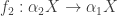
  if there is a continuous function
  such that
  . See the following figure.
 (partial order), which means that there is a continuous
  such that
  (the same point in
  is extendable to a continuous
  .
. illustrates that the
  can be regarded as
  where
where  is some closed and bounded interval. The
  . To this end, we need to produce a continuous function
  such that
  .
. , let
, let  . For each
  be the projection map from this cube into
  . Thus by assumption, each
  . Now define
  by the following:
 ,
,  such that
 , we have
  . Note that
  agrees with
  since
since  where
where  for each
  where
where  for each
 is dense in
  . Thus we have:

 can be extended to
  where
where  and
and  as topological spaces with the order topology derived from the well ordering of the ordinals. The space
  ,
,  (see result B in
  .
.
 , which is dense in
  is an arbitrary continuous function where
  such that
  is given in this previous post (
 ,
, ![I_g=[0,1]](https://s0.wp.com/latex.php?latex=I_g%3D%5B0%2C1%5D&bg=ffffff&fg=333333&s=0&c=20201002) . The map
. The map  is defined by:
 is the point
  such that
  for each
  coordinate of the point
  ).
).
 is a homeomorphism, see
  is the topological copy of
  .
.
 is written as
  .
. , where
  into
into  . We have the following diagram.
 . The rest of the proof is to define
  such that
  (i.e. the
  coordinate of
  coordinate of
 or
or  ). The following shows the derivation.


 . The following derivation shows that
  .
.
 . So it makes sense to define
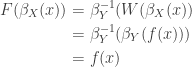
 and
and  is said to be a compactification of the space
  is a homeomorphism from
  , we have the Stone-Cech compactification
  , which is a subspace of the cube
  . The circle
  contains a copy of the real line
  and
and  ) if there exists a homeomorphism
 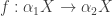 such that
  . In other words, the following diagram commutes.
 is mapped to
  .
. be the class of all compactifications of
  for compactifications.
 and
and  With
With  such that
 such that
 to
to  , we have
 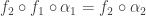 . Applying
  to this result, we have
 is a map from
  indicates that when
  , it is the identity map. Thus
  must equal to the identity map on
  This direction is straightforward. Let
  implies
  . By Theorem C1,
 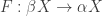 such that
  . The existence of the map
  . By the assumption that
  such that
  . The existence of
  or as a sequence
  such that each term (or coordinate)
 ![t_f \in I=[0,1]](https://s0.wp.com/latex.php?latex=t_f+%5Cin+I%3D%5B0%2C1%5D&bg=ffffff&fg=333333&s=0&c=20201002) .
. is the point in the cube such that for each
  . This map
 ![\Phi(x):\mathbb{R} \rightarrow [0,1]](https://s0.wp.com/latex.php?latex=%5CPhi%28x%29%3A%5Cmathbb%7BR%7D+%5Crightarrow+%5B0%2C1%5D&bg=ffffff&fg=333333&s=0&c=20201002) defined by:
defined by: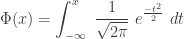
 is the cumulative distribution function (CDF) of the standard normal distribution. The following figure is the graph.
 and
and  , we cannot extend the function
  to a continuous function defined on
  defined on the open interval
  , which is a topological copy of
  to a continuous function defined on
  .
. , which maps
 ![[-1,1]](https://s0.wp.com/latex.php?latex=%5B-1%2C1%5D&bg=ffffff&fg=333333&s=0&c=20201002) . Based on Theorem C1,
. Based on Theorem C1,  can be extended to a function
 ![G: \beta \mathbb{R} \rightarrow [-1,1]](https://s0.wp.com/latex.php?latex=G%3A+%5Cbeta+%5Cmathbb%7BR%7D+%5Crightarrow+%5B-1%2C1%5D&bg=ffffff&fg=333333&s=0&c=20201002) .
. ![t \in [-1,1]](https://s0.wp.com/latex.php?latex=t+%5Cin+%5B-1%2C1%5D&bg=ffffff&fg=333333&s=0&c=20201002) , let
, let  . For example,
  is the set
  . Furthermore, for each
  , which is a compact set in
  for each
  is a discrete set in
  for each
  show that at minimum we are adding continuum many points to form
  ,
,  and
and  are disjoint (they are separated by disjoint open sets in
  ).
). , where