Revisiting example 106 from Steen and Seebach

Posted on December 25, 2021 by Dan Ma

The example 106 from Counterexamples in Topology by Steen and Seebach [3] is the space $\omega_1 \times I^I$ where the first factor $\omega_1$ is the space of countable ordinals with the usual order topology and the second factor $I^I$ is the product of continuum many copies of the unit interval $I=[0,1]$ .

This space was previously discussed in this site. One of the key results from that discussion is that $\omega_1 \times I^I$ is not normal, a result not shown in Steen and Seebach. The proof that was given in this site (see here) is based on an article published in 1976 [1], long before the publication date of the first edition of Steen and Seebach in 1970. It turns out that the non-normality of $\omega_1 \times I^I$ was given as an exercise in Steen and Seebach in the problem section at the end of the book (problem 127 in page 211, Dover edition). Problem 127: Show that $[0, \Omega) \times I^I$ is not normal. This indicates that the result not shown in Steen and Seebach was because it was given as a problem and not because the tool for solving it was not yet available. The fact that it is given as an exercise also means that there is a more basic proof of the non-normality of $\omega_1 \times I^I$ . So, once this is realized, I set out to find a simpler proof or at least one that does not rely on the result from [1]. Interestingly, this proof brings out a broader discussion that is worthwhile and goes beyond the example at hand. The goal here is to examine the more basic proof and the broader discussion.

A Classic Example

Before talking about the promised proof, we consider the product of $\omega_1$ and its immediate successor.

As noted at the beginning, the space $\omega_1$ is the set of all countable ordinals with the order topology. The ordinal $\omega_1+1$ is the immediate successor of $\omega_1$ . It can be regarded as the result of adding one more point to $\omega_1$ . The extra point is $\omega_1$ , i.e., $\omega_1 +1=\omega_1 \cup \{ \omega_1 \}$ with $\omega_1$ greater than all points $\beta < \omega_1$ . The ordinal $\omega_1+1$ with the order topology is a compact space. Using interval notation, $\omega_1=[0, \omega_1)$ and $\omega_1+1=[0, \omega_1]$ . As ordinals, $\omega_1$ is the first uncountable ordinal and $\omega_1+1$ is the first uncountable successor ordinal. For more information, see here.

The product $[0, \omega_1) \times [0, \omega_1]$ is a classic example of a product of a normal space (the first factor) and a compact space (the second factor) that is not normal. This example and others like it show that normality is easily broken upon taking product even if one of the factors is as nice as a compact space. The non-normality of $[0, \omega_1) \times [0, \omega_1]$ is discussed here. In that proof, two disjoint closed sets $H$ and $K$ are given such that they cannot be separated by disjoint open sets. The $H$ and $K$ are:

$H=\{ (\alpha, \alpha): \alpha < \omega_1 \}$

$K=\{(\alpha, \omega_1): \alpha < \omega_1 \}$

The Basic Proof

To show that $\omega_1 \times I^I$ is not normal, we show that one of its closed subspaces is not normal. That closed subspace is $[0, \omega_1) \times [0, \omega_1]$ . To this end, we show that $[0, \omega_1]$ can be embedded in the product space $I^I$ . With a non-normal closed subspace, it follows that $\omega_1 \times I^I$ is not normal. The remainder of the proof is to give the embedding.

We show that $[0, \omega_1]$ can be embedded as a closed subspace of $I^{\omega_1}$ , the product of $\omega_1$ many copies of $I$ . This means that $[0, \omega_1]$ is also a closed subspace of $I^I$ .

For each $\beta < \omega_1$ , define $T_\beta: \omega_1 \rightarrow I$ as follows:

$T_\beta(\gamma) = \begin{cases} 1 & \ \ \ \mbox{if } \gamma < \beta \\ 0 & \ \ \ \mbox{if } \gamma \ge \beta \end{cases}$

Furthermore, define $T: \omega_1 \rightarrow I$ by letting $T(\beta)=1$ for all $\beta < \omega_1$ . Consider the correspondence $\beta \rightarrow T_\beta$ with $\beta < \omega_1$ and $\omega_1 \rightarrow T$ . The mapping is clearly one-to-one from $[0, \omega_1]$ onto $\{ T_\beta: \beta < \omega_1 \} \cup \{ T \}$ . Upon closer inspection, the mapping in each direction is continuous (this is a good exercise to walk through). Thus, the mapping is a homeomorphism. It follows that $[0, \omega_1]$ can be considered a subspace of $I^{\omega_1}$ . Since $[0, \omega_1]$ is compact, it must be a closed subspace. With the cardinality of $\omega_1$ being less than or equal to continuum, it follows that $[0, \omega_1]$ can be embedded as a closed subspace of $I^I$ .

Stone-Cech Compactification

The first broader discussion is that of Stone-Cech compactification. More specifically, $\beta \omega_1=\omega_1+1$ , i.e., the Stone-Cech compactification of the first uncountable ordinal is its immediate successor.

To see that $\beta \omega_1=\omega_1+1$ , note that every continuous function defined on $[0,\omega_1)$ is bounded and is eventually constant (see result B here). As a result, every continuous function defined on $[0,\omega_1)$ can be extended to a continuous function defined on $[0, \omega_1]$ . For any continuous function $f: \omega_1 \rightarrow \mathbb{R}$ , we can simply define $f(\omega_1)$ to be the eventual constant value. A subspace $W$ of a space $Y$ is $C^*$ -embedded in $Y$ if every bounded continuous real-valued function on $W$ can be extended to $Y$ . According to theorem 19.12 in [4], if $Y$ is a compactification of $X$ and if $X$ is $C^*$ -embedded in $Y$ , then $Y$ is the Stone-Cech compactification of $X$ . Thus $[0,\omega_1)$ is $C^*$ -embedded in $[0,\omega_1]$ and $[0,\omega_1]$ is the Stone-Cech compactification of $[0,\omega_1)$ . In this instance, the Stone-Cech compactification agrees with the one-point compactification. Consider the following class theorem about normality in product space. The theorem is Corollary 3.4 in the chapter on products of normal spaces in the handbook of set-theoretic topology [2].

Theorem 1
Let $X$ be a space. The following conditions are equivalent.

The space $X$ is paracompact.
The product space $X \times \beta X$ is normal.

Based on the discussion presented above, the non-normality of $\omega_1 \times I^I$ is due to the non-normality of $[0, \omega_1) \times [0, \omega_1]$ . Based on this theorem, the non-normality of $[0, \omega_1) \times [0, \omega_1]$ is due to the non-paracompactness of $[0, \omega_1)$ . See result G here for a proof that $[0, \omega_1)$ is not paracompact.

The discussion up to this point points to two ways to prove that $\omega_1 \times I^I$ is not normal. One way is the basic proof indicated above. The other way is to use Theorem 1, along with the homeomorphic embedding from $[0, \omega_1]$ into $I^I$ , the fact that $\beta \omega_1=\omega_1+1$ and the fact that $[0, \omega_1)$ is not paracompact. Both are valuable. The first way is basic and is a constructive proof. Because it is more hands-on, it is a better proof to learn from. The second way provides a broader perspective that is informative but requires quoting a couple of fairly deep results. Perhaps it is best used as a second proof for perspective.

Countable Tightness

The essence of the basic proof above goes like this: if the space $Y$ contains a copy of $\omega_1+1=[0, \omega_1]$ , then the product space $[0, \omega_1) \times Y$ is not normal. The contrapositive statement would be the following:

Corollary
Let $Y$ be a space. If the product space $\omega_1 \times Y$ is normal, then $Y$ cannot contain a copy of $\omega_1+1$ .

In the space of $\omega_1+1=[0, \omega_1]$ , note the following about the last point: $\omega_1 \in \overline{[0, \omega_1)}$ but $\omega_1 \notin \overline{C}$ for any countable $C \subset [0, \omega_1)$ , i.e., the last point is the limit point of the set of all the points preceding it but is not in the closure of any countable set. This means that the space $\omega_1+1=[0, \omega_1]$ does not have countable tightness (or is not countably tight). See here for definition. The property of countable tightness is hereditary. If $Y$ contains a copy of $\omega_1+1$ , then $Y$ is not countably tight (or is uncountably tight). This brings us to the following theorem.

Theorem 2
Let $Y$ be an infinite compact space. Then $\omega_1 \times Y$ is normal if and only if $Y$ has countable tightness.

Whenever we consider the normality of a product with the first factor being $\omega_1$ and the second factor being a compact space, the real story is the tightness of that compact space. If the tightness is countable, the product is normal. Otherwise, the product is not normal. The theorem is another reason that $\omega_1 \times I^I$ is not normal. Instead of embedding $[0, \omega_1]$ into $I^I$ , we can actually show that $I^I$ does not have countable tightness. This is the approach that was taken in this previous post.

Theorem 2 is the result from 1976 alluded to earlier [1]. A proof of Theorem 2 is found in this previous post. For results concerning normality in a product space with a compact factor (the other factor does not have to be $\omega_1$ ), see the chapter on products of normal spaces in the handbook of set-theoretic topology [2].

Reference

Nogura, T., Tightness of compact Hausdorff space and normality of product spaces, J. Math. Soc. Japan, 28, 360-362, 1976.
Przymusinski T. C., Products of Normal Spaces, Handbook of Set-Theoretic Topology (K. Kunen and J. E. Vaughan, eds), Elsevier Science Publishers B. V., Amsterdam, 781-826, 1984.
Steen, L. A., Seebach, J. A., Counterexamples in Topology, Dover Publications, Inc., New York, 1995.
Willard, S., General Topology, Addison-Wesley Publishing Company, 1970.

$\text{ }$

Dan Ma topology

Daniel Ma topology

Dan Ma math

Daniel Ma mathematics

$\copyright$ 2021 – Dan Ma

Michael line and Morita’s conjectures

Posted on September 9, 2018 by Dan Ma

This post discusses Michael line from the point of view of the three conjectures of Kiiti Morita.

K. Morita defined the notion of P-spaces in [7]. The definition of P-spaces is discussed here in considerable details. K. Morita also proved that a space $X$ is a normal P-space if and only if the product $X \times Y$ is normal for every metrizable space $Y$ . As a result of this characterization, the notion of normal P-space (a space that is a normal space and a P-space) is useful in the study of products of normal spaces. Just to be clear, we say a space is a non-normal P-space (i.e. a space that is not a normal P-space) if the space is a normal space that is not a P-space.

K. Morita formulated his three conjectures in 1976. The statements of the conjectures are given below. Here is a basic discussion of the three conjectures. The notion of normal P-spaces is a theme that runs through the three conjectures. The conjectures are actually theorems since 2001 [2].

Here’s where Michael line comes into the discussion. Based on the characterization of normal P-spaces mentioned above, to find a normal space that is not a P-space (a non-normal P-space), we would need to find a non-normal product $X \times Y$ such that one of the factors is a metric space and the other factor is a normal space. The first such example in ZFC is from an article by E. Michael in 1963 (found here and here). In this example, the normal space is $M$ , which came be known as the Michael line, and the metric space is $\mathbb{P}$ , the space of irrational numbers (as a subspace of the real line). Their product $M \times \mathbb{P}$ is not normal. A basic discussion of the Michael line is found here.

Because $M \times \mathbb{P}$ is not normal, the Michael line $M$ is not a normal P-space. Prior to E. Michael’s 1963 article, we have to reach back to 1955 to find an example of a non-normal product where one factor is a metric space. In 1955, M. E. Rudin used a Souslin line to construct a Dowker space, which is a normal space whose product with the closed unit interval is not normal. The existence of a Souslin line was shown to be independent of ZFC in the late 1960s. In 1971, Rudin constructed a Dowker space in ZFC. Thus finding a normal space that is not a normal P-space (finding a non-normal product $X \times Y$ where one factor is a metric space and the other factor is a normal space) is not a trivial matter.

Morita’s Three Conjectures

We show that the Michael line illustrates perfectly the three conjectures of K. Morita. Here’s the statements.

Morita’s Conjecture I. Let $X$ be a space. If the product $X \times Y$ is normal for every normal space $Y$ then $X$ is a discrete space.

Morita’s Conjecture II. Let $X$ be a space. If the product $X \times Y$ is normal for every normal P-space $Y$ then $X$ is a metrizable space.

Morita’s Conjecture III. Let $X$ be a space. If the product $X \times Y$ is normal for every normal countably paracompact space $Y$ then $X$ is a metrizable $\sigma$ -locally compact space.

The contrapositive statement of Morita’s conjecture I is that for any non-discrete space $X$ , there exists a normal space $Y$ such that $X \times Y$ is not normal. Thus any non-discrete space is paired with a normal space for forming a non-normal product. The Michael line $M$ is paired with the space of irrational numbers $\mathbb{P}$ . Obviously, the space $\mathbb{P}$ is paired with the Michael line $M$ .

The contrapositive statement of Morita’s conjecture II is that for any non-metrizable space $X$ , there exists a normal P-space $Y$ such that $X \times Y$ is not normal. The pairing is more specific than for conjecture I. Any non-metrizable space is paired with a normal P-space to form a non-normal product. As illustration, the Michael line $M$ is not metrizable. The space $\mathbb{P}$ of irrational numbers is a metric space and hence a normal P-space. Here, $M$ is paired with $\mathbb{P}$ to form a non-normal product.

The contrapositive statement of Morita’s conjecture III is that for any space $X$ that is not both metrizable and $\sigma$ -locally compact, there exists a normal countably paracompact space $Y$ such that $X \times Y$ is not normal. Note that the space $\mathbb{P}$ is not $\sigma$ -locally compact (see Theorem 4 here). The Michael line $M$ is paracompact and hence normal and countably paracompact. Thus the metric non- $\sigma$ -locally compact $\mathbb{P}$ is paired with normal countably paracompact $M$ to form a non-normal product. Here, the metric space $\mathbb{P}$ is paired with the non-normal P-space $M$ .

In each conjecture, each space in a certain class of spaces is paired with one space in another class to form a non-normal product. For Morita’s conjecture I, each non-discrete space is paired with a normal space. For conjecture II, each non-metrizable space is paired with a normal P-space. For conjecture III, each metrizable but non- $\sigma$ -locally compact is paired with a normal countably paracompact space to form a non-normal product. Note that the paired normal countably paracompact space would be a non-normal P-space.

Michael line as an example of a non-normal P-space is a great tool to help us walk through the three conjectures of Morita. Are there other examples of non-normal P-spaces? Dowker spaces mentioned above (normal spaces whose products with the closed unit interval are not normal) are non-normal P-spaces. Note that conjecture II guarantees a normal P-space to match every non-metric space for forming a non-normal product. Conjecture III guarantees a non-normal P-space to match every metrizable non- $\sigma$ -locally compact space for forming a non-normal product. Based on the conjectures, examples of normal P-spaces and non-normal P-spaces, though may be hard to find, are guaranteed to exist.

We give more examples below to further illustrate the pairings for conjecture II and conjecture III. As indicated above, non-normal P-spaces are hard to come by. Some of the examples below are constructed using additional axioms beyond ZFC. The additional examples still give an impression that the availability of non-normal P-spaces, though guaranteed to exist, is limited.

Examples of Normal P-Spaces

One example is based on this classic theorem: for any normal space $X$ , $X$ is paracompact if and only if the product $X \times \beta X$ is normal. Here $\beta X$ is the Stone-Cech compactification of the completely regular space $X$ . Thus any normal but not paracompact space $X$ (a non-metrizable space) is paired with $\beta X$ , a normal P-space, to form a non-normal product.

Naturally, the next class of non-metrizable spaces to be discussed should be the paracompact spaces that are not metrizable. If there is a readily available theorem to provide a normal P-space for each non-metrizable paracompact space, then there would be a simple proof of Morita’s conjecture II. The eventual solution of conjecture II is far from simple [2]. We narrow the focus to the non-metrizable compact spaces.

Consider this well known result: for any infinite compact space $X$ , the product $\omega_1 \times X$ is normal if and only if the space $X$ has countable tightness (see Theorem 1 here). Thus any compact space with uncountable tightness is paired with $\omega_1$ , the space of all countable ordinals, to form a non-normal product. The space $\omega_1$ , being a countably compact space, is a normal P-space. A proof that normal countably compact space is a normal P-space is given here.

We now handle the case for non-metrizable compact spaces with countable tightness. In this case, compactness is not needed. For spaces with countable tightness, consider this result: every space with countable tightness, whose products with all perfectly normal spaces are normal, must be metrizable [3] (see Corollary 7). Thus any non-metrizable space with countable tightness is paired with some perfectly normal space to form a non-normal product. Any reader interested in what these perfectly normal spaces are can consult [3]. Note that perfectly normal spaces are normal P-spaces (see here for a proof).

Examples of Non-Normal P-Spaces

Another non-normal product is $X_B \times B$ where $B \subset \mathbb{R}$ is a Bernstein set and $X_B$ is the space with the real line as the underlying set such that points in $B$ are isolated and points in $\mathbb{R}-B$ retain the usual open sets. The set $B \subset \mathbb{R}$ is said to be a Bernstein set if every uncountable closed subset of the real line contains a point in B and contains a point in the complement of B. Such a set can be constructed using transfinite induction as shown here. The product $X_B \times B$ is not normal where $B$ is considered a subspace of the real line. The proof is essentially the same proof that shows $M \times \mathbb{P}$ is not normal (see here). The space $X_B$ is a Lindelof space. It is not a normal P-space since its product with $B$ , a separable metric space, is not normal. However, this example is essentially the same example as the Michael line since the same technique and proof are used. On the one hand, the $X_B \times B$ example seems like an improvement over Michael line example since the first factor $X_B$ is Lindelof. On the other hand, it is inferior than the Michael line example since the second factor $B$ is not completely metrizable.

Moving away from the idea of Michael, there exist a Lindelof space and a completely metrizable (but not separable) space whose product is of weight $\omega_1$ and is not normal [5]. This would be a Lindelof space that is a non-normal P-space. However, this example is not as elementary as the Michael line, making it not as effective as an illustration of Morita’s three conjectures.

The next set of non-normal P-spaces requires set theory. A Michael space is a Lindelof space whose product with $\mathbb{P}$ , the space of irrational numbers, is not normal. Michael problem is the question: is there a Michael space in ZFC? It is known that a Michael space can be constructed using continuum hypothesis [6] or using Martin’s axiom [1]. The construction using continuum hypothesis has been discussed in this blog (see here). The question of whether there exists a Michael space in ZFC is still unsolved.

The existence of a Michael space is equivalent to the existence of a Lindelof space and a separable completely metrizable space whose product is non-normal [4]. A Michael space, in the context of the discussion in this post, is a non-normal P-space.

The discussion in this post shows that the example of the Michael line and other examples of non-normal P-spaces are useful tools to illustrate Morita’s three conjectures.

Reference

Alster K.,On the product of a Lindelof space and the space of irrationals under Martin’s Axiom, Proc. Amer. Math. Soc., Vol. 110, 543-547, 1990.
Balogh Z.,Normality of product spaces and Morita’s conjectures, Topology Appl., Vol. 115, 333-341, 2001.
Chiba K., Przymusinski T., Rudin M. E.Nonshrinking open covers and K. Morita’s duality conjectures, Topology Appl., Vol. 22, 19-32, 1986.
Lawrence L. B., The influence of a small cardinal on the product of a Lindelof space and the irrationals, Proc. Amer. Math. Soc., 110, 535-542, 1990.
Lawrence L. B., A ZFC Example (of Minimum Weight) of a Lindelof Space and a Completely Metrizable Space with a Nonnormal Product, Proc. Amer. Math. Soc., 124, No 2, 627-632, 1996.
Michael E., Paracompactness and the Lindelof property in nite and countable cartesian products, Compositio Math., 23, 199-214, 1971.
Morita K., Products of Normal Spaces with Metric Spaces, Math. Ann., Vol. 154, 365-382, 1964.
Rudin M. E., A Normal Space $X$ for which $X \times I$ is not Normal, Fund. Math., 73, 179-186, 1971.

$\text{ }$

Dan Ma math

Daniel Ma mathematics

$\copyright$ 2018 – Dan Ma

Three conjectures of K Morita

Posted on August 28, 2018 by Dan Ma

This post discusses the three conjectures that were proposed by K. Morita in 1976. These conjectures concern normality in product spaces. To start the discussion, here’s the conjectures.

Morita’s Conjecture I. Let $X$ be a space. The product $X \times Y$ is normal for every normal space $Y$ if and only if $X$ is a discrete space.

Morita’s Conjecture II. Let $X$ be a space. The product $X \times Y$ is normal for every normal P-space $Y$ if and only if $X$ is a metrizable space.

Morita’s Conjecture III. Let $X$ be a space. The product $X \times Y$ is normal for every normal countably paracompact space $Y$ if and only if $X$ is a metrizable $\sigma$ -locally compact space.

These statements are no longer conjectures. Partial results appeared after the conjectures were proposed in 1976. The complete resolution of the conjectures came in 2001 in a paper by Zoli Balogh [5]. Though it is more appropriate to call these statements theorems, it is still convenient to call them conjectures. Just know that they are now known results rather open problems to be solved. The focus here is not on the evolution of the solutions. Instead, we discuss the relations among the three conjectures and why they are amazing results in the study of normality in product spaces.

As discussed below, in each of these conjectures, one direction is true based on prior known theorems (see Theorem 1, Theorem 2 and Theorem 4 below). The conjectures can be stated as follows.

Morita’s Conjecture I. Let $X$ be a space. If the product $X \times Y$ is normal for every normal space $Y$ then $X$ is a discrete space.

Morita’s Conjecture II. Let $X$ be a space. If the product $X \times Y$ is normal for every normal P-space $Y$ then $X$ is a metrizable space.

Morita’s Conjecture III. Let $X$ be a space. If the product $X \times Y$ is normal for every normal countably paracompact space $Y$ then $X$ is a metrizable $\sigma$ -locally compact space.

P-spaces are defined by K. Morita [11]. He proved that a space $X$ is a normal P-space if and only if the product $X \times Y$ is normal for every metrizable space $Y$ (see theorem 2 below). Normal P-spaces are also discussed here. A space $X$ is $\sigma$ -locally compact space if $X$ is the union of countably many locally compact subspaces each of which is also closed subspace of $X$ .

As we will see below, these conjectures are also called duality conjectures because they are duals of known results.

[2] is a survey of Morita’s conjecture.

Duality Conjectures

Here’s three theorems that are duals to the conjectures.

Theorem 1
Let $X$ be a space. The product space $X \times Y$ is normal for every discrete space $Y$ if and only if $X$ is normal.

Theorem 2
Let $X$ be a space. The product space $X \times Y$ is normal for every metrizable space $Y$ if and only if $X$ is a normal P-space.

Theorem 3
Let $X$ be a space. The product space $X \times Y$ is normal for every metrizable $\sigma$ -locally compact space $Y$ if and only if $X$ is normal countably paracompact.

The key words in red are for emphasis. In each of these three theorems, if we switch the two key words in red, we would obtain the statements for the conjectures. In this sense, the conjectures are called duality conjectures since they are duals of known results.

Theorem 1 is actually not found in the literature. It is an easy theorem. Theorem 2, found in [11], is a characterization of normal P-space (discussed here). Theorem 3 is a well known result based on the following theorem by K. Morita [10].

Theorem 4
Let $Y$ be a metrizable space. Then the product $X \times Y$ is normal for every normal countably paracompact space $X$ if and only if $Y$ is a $\sigma$ -locally compact space.

We now show that Theorem 3 can be established using Theorem 4. Theorem 4 is also Theorem 3.5 in p. 111 of [2]. A proof of Theorem 4 is found in Theorem 1.8 in p. 130 of [8].

Proof of Theorem 3
$\Longleftarrow$ Suppose $X$ is normal and countably paracompact. Let $Y$ be a metrizable $\sigma$ -locally compact space. By Theorem 4, $X \times Y$ is normal.

$\Longrightarrow$ This direction uses Dowker’s theorem. We give a contrapositive proof. Suppose that $X$ is not both normal and countably paracompact. Case 1. $X$ is not normal. Then $X \times \{ y \}$ is not normal where $\{ y \}$ is any one-point discrete space. Case 2. $X$ is normal and not countably paracompact. This means that $X$ is a Dowker space. Then $X \times [0,1]$ is not normal. In either case, $X \times Y$ is not normal for some compact metric space. Thus $X \times Y$ is not normal for some $\sigma$ -locally compact metric space. This completes the proof of Theorem 3. $\square$

The First and Third Conjectures

The first conjecture of Morita was proved by Atsuji [1] and Rudin [13] in 1978. The proof in [13] is a constructive proof. The key to that solution is to define a $\kappa$ -Dowker space. Suppose $X$ is a non-discrete space. Let $\kappa$ be the least cardinal of a non-discrete subspace of $X$ . Then construct a $\kappa$ -Dowker space $Y$ as in [13]. It follows that $X \times Y$ is not normal. The proof that $X \times Y$ is not normal is discussed here.

Conjecture III was confirmed by Balogh in 1998 [4]. We show here that the first and third conjectures of Morita can be confirmed by assuming the second conjecture.

Conjecture II implies Conjecture I
We give a contrapositive proof of Conjecture I. Suppose that $X$ is not discrete. We wish to find a normal space $Y$ such that $X \times Y$ is not normal. Consider two cases for $X$ . Case 1. $X$ is not metrizable. By Conjecture II, $X \times Y$ is not normal for some normal P-space $Y$ . Case 2. $X$ is metrizable. Since $X$ is infinite and metric, $X$ would contain an infinite compact metric space $S$ . For example, $X$ contains a non-trivial convergent sequence and let $S$ be a convergence sequence plus the limit point. Let $Y$ be a Dowker space. Then the product $S \times Y$ is not normal. It follows that $X \times Y$ is not normal. Thus there exists a normal space $Y$ such that $X \times Y$ is not normal in either case. $\square$

Conjecture II implies Conjecture III
Suppose that the product $X \times Y$ is normal for every normal and countably paracompact space $Y$ . Since any normal P-space is a normal countably paracompact space, $X \times Y$ is normal for every normal and P-space $Y$ . By Conjecture II, $X$ is metrizable. By Theorem 4, $X$ is $\sigma$ -locally compact. $\square$

The Second Conjecture

The above discussion shows that a complete solution to the three conjectures hinges on the resolution of the second conjecture. A partial resolution came in 1986 [6]. In that paper, it was shown that under V = L, conjecture II is true.

The complete solution of the second conjecture is given in a paper of Balogh [5] in 2001. The path to Balogh’s proof is through a conjecture of M. E. Rudin identified as Conjecture 9.

Rudin’s Conjecture 9. There exists a normal P-space $X$ such that some uncountable increasing open cover of $X$ cannot be shrunk.

Conjecture 9 was part of a set of 14 conjectures stated in [14]. It is also discussed in [7]. In [6], conjecture 9 was shown to be equivalent to Morita’s second conjecture. In [5], Balogh used his technique for constructing a Dowker space of cardinality continuum to obtain a space as described in conjecture 9.

The resolution of conjecture II is considered to be one of Balogh greatest hits [3].

Abundance of Non-Normal Products

One immediate observation from Morita’s conjecture I is that existence of non-normal products is wide spread. Conjecture I indicates that every normal non-discrete space $X$ is paired with some normal space $Y$ such that their product is not normal. So every normal non-discrete space forms a non-normal product with some normal space. Given any normal non-discrete space (no matter how nice it is or how exotic it is), it can always be paired with another normal space (sometimes paired with itself) for a non-normal product.

Suppose we narrow the focus to spaces that are normal and non-metrizable. Then any such space $X$ is paired with some normal P-space $Y$ to form a non-normal product space (Morita’s conjecture II). By narrowing the focus on $X$ to the non-metrizable spaces, we obtain more clarity on the paired space to form non-normal product, namely a normal P-space. As an example, let $X$ be the Michael line (normal and non-metrizable). It is well known that $X$ in this case is paired with $\mathbb{P}$ , the space of irrational numbers with the usual Euclidean topology, to form a non-normal product (discussed here).

Another example is $X$ being the Sorgenfrey line. It is well known that $X$ in this case is paired with itself to form a non-normal product (discussed here). Morita’s conjectures are powerful indication that these two non-normal products are not isolated phenomena.

Another interesting observation about conjecture II is that normal P-spaces are not productive with respect to normality. More specifically, for any non-metrizable normal P-space $X$ , conjecture II tells us that there exists another normal P-space $Y$ such that $X \times Y$ is not normal.

Now we narrow the focus to spaces that are metrizable but not $\sigma$ -locally compact. For any such space $X$ , conjecture III tells us that $X$ is paired with a normal countably paracompact space $Y$ to form a non-normal product. Using the Michael line example, this time let $X=\mathbb{P}$ , the space of irrational numbers, which is a metric space that is not $\sigma$ -locally compact. The paired normal and countably paracompact space $Y$ is the Michael line.

Each conjecture is about existence of a normal $Y$ that is paired with a given $X$ to form a non-normal product. For Conjecture I, the given $X$ is from a wide class (normal non-discrete). As a result, there is not much specific information on the paired $Y$ , other than that it is normal. For Conjectures II and III, the given space $X$ is from narrower classes. As a result, there is more information on the paired $Y$ .

The concept of Dowker spaces runs through the three conjectures, especially the first conjecture. Dowker spaces and $\kappa$ -Dowker spaces provide reliable pairing for non-normal products. In fact this is one way to prove conjecture I [13], also see here. For any normal space $X$ with a countable non-discrete subspace, the product of $X$ and any Dowker space is not normal (discussed here). For any normal space $X$ such that the least cardinality of a non-discrete subspace is an uncountable cardinal $\kappa$ , the product $X \times Y$ is not normal where $Y$ is a $\kappa$ -Dowker space as constructed in [13], also discussed here.

In finding a normal pair $Y$ for a normal space $X$ , if we do not care about $Y$ having a high degree of normal productiveness (e.g. normal P or normal countably paracompact), we can always let $Y$ be a Dowker space or $\kappa$ -Dowker space. In fact, if the starting space $X$ is a metric space, the normal pair for a non-normal product (by definition) has to be a Dowker space. For example, if $X=[0,1]$ , then the normal space $Y$ such that $X \times Y$ is by definition a Dowker space. The search for a Dowker space spanned a period of 20 years. For the real line $\mathbb{R}$ , the normal pair for a non-normal product is also a Dowker space. For “nice” spaces such as metric spaces, finding a normal space to form non-normal product is no trivial problem.

Reference

Atsuji M.,On normality of the product of two spaces, General Topology and Its Relation to Modern Analysis and Algebra (Proc. Fourth Prague Topology sympos., 1976), Part B, 25–27, 1977.
Atsuji M.,Normality of product spaces I, in: K. Morita, J. Nagata (Eds.), Topics in General
Topology, North-Holland, Amsterdam, 81–116, 1989.
Burke D., Gruenhage G.,Zoli, Top. Proc., Vol. 27, No 1, i-xxii, 2003.
Balogh Z.,Normality of product spaces and K. Morita’s third conjecture, Topology Appl., Vol. 84, 185-198, 1998.
Balogh Z.,Normality of product spaces and Morita’s conjectures, Topology Appl., Vol. 115, 333-341, 2001.
Chiba K., Przymusinski T., Rudin M. E.Nonshrinking open covers and K. Morita’s duality conjectures, Topology Appl., Vol. 22, 19-32, 1986.
Gruenhage G.,Mary Ellen’s Conjectures,, Special Issue honoring the memory of Mary Ellen Rudin, Topology Appl., Vol. 195, 15-25, 2015.
Hoshina T.,Normality of product spaces II, in: K. Morita, J. Nagata (Eds.), Topics in General Topology, North-Holland, Amsterdam, 121–158, 1989.
Morita K., On the Product of a Normal Space with a Metric Space, Proc. Japan Acad., Vol. 39, 148-150, 1963. (article information; paper)
Morita K., Products of Normal Spaces with Metric Spaces II, Sci. Rep. Tokyo Kyoiku Dagaiku Sec A, 8, 87-92, 1963.
Morita K., Products of Normal Spaces with Metric Spaces, Math. Ann., Vol. 154, 365-382, 1964.
Morita K., Nagata J., Topics in General Topology, Elsevier Science Publishers, B. V., The Netherlands, 1989.
Rudin M. E., $\kappa$ -Dowker Spaces, Czechoslovak Mathematical Journal, 28, No.2, 324-326, 1978.
Rudin M. E., Some conjectures, in: Open Problems in Topology, J. van Mill and G.M. Reed,
eds., North Holland, 184–193, 1990.
Telgárski R., A characterization of P-spaces, Proc. Japan Acad., Vol. 51, 802–807, 1975.

$\text{ }$

Dan Ma math

Daniel Ma mathematics

$\copyright$ 2018 – Dan Ma

Extracting more information from Dowker’s theorem

Posted on May 1, 2017 by Dan Ma

Countably paracompact spaces are discussed in a previous post. The discussion of countably paracompactness in the previous post is through discussing Dowker’s theorem. In this post, we discuss a few more facts that can be derived from Dowker’s theorem.

____________________________________________________________________

Dowker’s Theorem

Essentially, Dowker’s theorem is the statement that for a normal space $X$ , the space $X$ is countably paracompact if any only if $X \times Y$ is normal for any infinite compact metric space. The following is the full statement of Dowker’s theorem. The long list of equivalent conditions is important for applications in various scenarios.

Theorem 1 (Dowker’s Theorem)
Let $X$ be a normal space. The following conditions are equivalent.

The space $X$ is countably paracompact.
Every countable open cover of $X$ has a point-finite open refinement.
If $\left\{U_n: n=1,2,3,\cdots \right\}$ is an open cover of $X$ , there exists an open refinement $\left\{V_n: n=1,2,3,\cdots \right\}$ such that $\overline{V_n} \subset U_n$ for each $n$ .
The product space $X \times Y$ is normal for any infinite compact metric space $Y$ .
The product space $X \times [0,1]$ is normal where $[0,1]$ is the closed unit interval with the usual Euclidean topology.
The product space $X \times S$ is normal where $S$ is a non-trivial convergent sequence with the limit point. Note that $S$ can be taken as a space homeomorphic to $\left\{1,\frac{1}{2},\frac{1}{3},\cdots \right\} \cup \left\{0 \right\}$ with the Euclidean topology.
For each sequence $\left\{A_n \subset X: n=1,2,3,\cdots \right\}$ of closed subsets of $X$ such that $A_1 \supset A_2 \supset A_3 \supset \cdots$ and $\cap_n A_n=\varnothing$ , there exist open sets $B_1,B_2,B_3,\cdots$ such that $A_n \subset B_n$ for each $n$ such that $\cap_n B_n=\varnothing$ .

A Dowker space is any normal space that is not countably paracompact. The notion of Dowker space was motivated by Dowker’s theorem since such a space would be a normal space $X$ for which $X \times [0,1]$ is not normal. The search for such a space took about 20 years from 1951 when C. H. Dowker proved the theorem to 1971 when M. E. Rudin constructed a ZFC example of a Dowker space.

Theorem 1 (Dowker’s theorem) is proved here and is further discussed in this previous post on countably paracompact space. The statement appears in Condition 6 here is not found in the previous version of the theorem. However, no extra effort is required to support it. Condition 5 trivially implies condition 6. The proof of condition 5 implying condition 7 (the proof of 4 implies 5 shown here) only requires that the product of $X$ and a convergent sequence is normal. So inserting condition 6 does not require extra proof.

____________________________________________________________________

Getting More from Dowker’s Theorem

As a result of Theorem 1, normal countably paracompact spaces are productive in normality with respect to compact metric spaces (condition 4 in Dowker’s theorem as stated above). Another way to look at condition 4 is that the normality in the product $X \times Y$ is a strong property. Whenever the product $X \times Y$ is normal, we know that each factor is normal. Dowker’s theorem tells us that whenever $X \times Y$ is normal and one of the factor is a compact metric space such as the unit interval $[0,1]$ , the other factor is countably paracompact. The fact can be extended. Even if the factors are not metric spaces, as long as one of the factors has a non-discrete point with “countable” tightness, normality of the product confers countably paracompactness on one of the factors. The following two theorems make this clear.

Theorem 2
Suppose that the product $X \times Y$ is normal. If one of the factor contains a non-trivial convergent sequence, then the other factor is countably paracompact.

Proof of Theorem 2
Suppose $Y$ contains a non-trivial convergent sequence. Let this sequence be denoted by $S =\left\{ x_n:n=1,2,3,\cdots \right\} \cup \left\{x \right\}$ such that the point $x$ is the limit point. Since $X \times Y$ is normal, both $X$ and $Y$ are normal and that $X \times S$ is normal. By Theorem 1, $X$ is countably paracompact. $\square$

Theorem 3
Suppose that the product $X \times Y$ is normal. If one of the factor contains a countable subset that is non-discrete, then the other factor is countably paracompact.

Proof of Theorem 3
To discuss this fact, we need to turn to the generalized Dowker’s theorem, which is Theorem 2 in this previous post. We will not re-state the theorem. The crucial direction is $7 \longrightarrow 4$ in that theorem. To avoid confusion, we call these two conditions A7 and A4. The following are the conditions.

$X \times Y$

$Y$

$\kappa$

$\left\{F_\alpha: \alpha<\kappa \right\}$

$X$

$\bigcap_{\alpha<\kappa} F_\alpha=\varnothing$

$\left\{G_\alpha: \alpha<\kappa \right\}$

$X$

$\bigcap_{\alpha<\kappa} G_\alpha=\varnothing$

$F_\alpha \subset G_\alpha$

$\alpha<\kappa$

Actually the proof in the previous post shows that A7 implies another condition that is equivalent to A4 for any infinite cardinal $\kappa$ . In particular, A7 $\longrightarrow$ A4 would hold for the countably infinite $\kappa=\omega$ . Note that under $\kappa=\omega$ , A4 would be the same as condition 7 in Theorem 1 above.

Thus by Theorem 2 in this previous post for the countably infinite case and by Theorem 1 in this post, the theorem is established. $\square$

Remarks
In Theorem 2, the second factor $Y$ does not have to be a metric space. As long as it has a non-trivial convergent sequence, the normality of the product (a big if in some situation) implies countably paracompactness in the other factor.

Theorem 3 is essentially a corollary of the proof of Theorem 2 in the previous post. One way to look at Theorem 3 is that the normality of the product $X \times Y$ is a strong statement. If the product is normal and if one factor has a countable non-discrete subspace, then the other factor is countably paracompact. Another way to look at it is through the angle of Dowker spaces. By Dowker’s theorem (Theorem 1), the product of any Dowker space with any infinite compact metric space is not normal. The pathology is actually more severe. A Dowker space is severely lacking in ability to form normal product, as the following corollary makes clear.

Corollary 4
If $X$ is a Dowker space, then $X \times Y$ is not normal for any space $Y$ containing a non-discrete countable subspace.

____________________________________________________________________

More Results

Two more results are discussed. According to Dowker’s theorem, the product of a countably paracompact space $X$ and any compact metric space is normal. In particular, $X \times [0,1]$ is normal. Theorem 5 is saying that with a little extra work, it can be shown that $X \times \mathbb{R}$ is normal. What makes this works is that the metric factor is $\sigma$ -compact.

Theorem 5
Let $X$ be a normal space. The following conditions are equivalent.

The space $X$ is countably paracompact.
The product space $X \times Y$ is normal for any non-discrete $\sigma$ -compact metric space $Y$ .
The product space $X \times \mathbb{R}$ is normal where $\mathbb{R}$ is the real number line with the usual Euclidean topology.

Proof of Theorem 5
$1 \rightarrow 2$
Suppose that $X$ is countably paracompact. Let $Y=\bigcup_{j=1}^\infty Y_j$ where each $Y_j$ is compact. Since $Y$ is a $\sigma$ -compact metric space, it is Lindelof. The Lindelof number and the weight agree in a metric space. Thus $Y$ has a countable base. According to Urysohn’s metrization theorem (discussed here), $Y$ can be embedded into the compact metric space $\prod_{j=1}^\infty W_j$ where each $W_j=[0,1]$ . For convenience, we consider $Y$ as a subspace of $\prod_{j=1}^\infty W_j$ . Furthermore, $X \times Y=\bigcup_{j=1}^\infty (X \times Y_j) \subset X \times\prod_{j=1}^\infty W_j$ .

By Theorem 1, each $X \times Y_j$ is normal and that $X \times\prod_{j=1}^\infty W_j$ is normal. Note that $X \times Y$ is an $F_\sigma$ -subset of the normal space $X \times\prod_{j=1}^\infty W_j$ . Since normality is passed to $F_\sigma$ -subsets, $X \times Y$ is normal.

Note. For a proof that $F_\sigma$ -subsets of normal spaces are normal, see 2.7.2(b) on p. 112 of Englelking [1].

$2 \rightarrow 3$ is immediate.

$3 \rightarrow 1$
Suppose that $X \times \mathbb{R}$ is normal. Then $X \times [0,1]$ is normal since it is a closed subspace of $X \times \mathbb{R}$ . By Theorem 1, $X$ is countably paracompact. $\square$

Theorem 6
Let $X$ be a normal space. Let $Y$ be a non-discrete $\sigma$ -compact metric space. Then $X \times Y$ is a normal space if and only if $X \times Y$ is countably paracompact.

Proof of Theorem 6
Let $Y=\bigcup_{j=1}^\infty Y_j$ where each $Y_j$ is compact. As in the proof of Theorem 5, we use the compact metric space $\prod_{j=1}^\infty W_j$ where each $W_j=[0,1]$ .

Suppose that $X \times Y$ is normal. Since $Y$ is a non-discrete metric space, $Y$ contains a countable non-discrete subspace. Then by either Theorem 2 or Theorem 3, $X$ is countably paracompact.

By Theorem 1, $X \times\prod_{j=1}^\infty W_j$ is normal. Note that $X \times \prod_{j=1}^\infty W_j \times [0,1]$ is normal since $(\prod_{j=1}^\infty W_j) \times [0,1]$ is a compact metric space. By Theorem 1 again, $X \times\prod_{j=1}^\infty W_j$ is countably paracompact.

As in the proof of Theorem 5, we can consider $Y$ as a subspace of $\prod_{j=1}^\infty W_j$ . Furthermore, $X \times Y=\bigcup_{j=1}^\infty X \times Y_j \subset X \times\prod_{j=1}^\infty W_j$ .

Note that $X \times Y$ is $F_\sigma$ -subset of the countably paracompact space $X \times\prod_{j=1}^\infty W_j$ . Since countably paracompactness is passed to $F_\sigma$ -subsets, we conclude that $X \times Y$ is countably paracompact.

Note. For a proof that countably paracompactness is passed to $F_\sigma$ -subsets, see the proof that paracompactness is passed to $F_\sigma$ -subsets in this previous post. Just apply the same proof but start with a countable open cover.

For the other direction, suppose that $X \times Y$ is countably paracompact. Since $X \times \left\{y \right\}$ is a closed subspace of $X \times Y$ with $y \in Y$ and is a copy of $X$ , $X$ is countably paracompact. Then by Theorem 5, $X \times Y$ is a normal space. $\square$

Remarks
Theorem 5 seems like an extension of Theorem 1. But the amount of extra work is very little. So normal countably paracompact spaces are productive with not just compact metric spaces but also with $\sigma$ -compact metric spaces. The $\sigma$ -compactness is absolutely crucial. The product of a normal countably paracompact space with a metric space does not have to be normal. For example, the Michael line $\mathbb{M}$ is paracompact and thus countably paracompact. The product of $\mathbb{M}$ and metric space is not necessarily normal (discussed here). However, the product of $\mathbb{M}$ and $\mathbb{R}$ or other $\sigma$ -compact metric space is normal.

Recall that a space is called a Dowker space if it is normal and not countably paracompact. For the type of product $X \times Y$ discussed in Theorem 6, it cannot be Dowker (if it is normal, it is countably paracompact). The two notions are the same with such product $X \times Y$ . Theorem 6 actually holds for a wider class than indicated. The following is Corollary 4.3 in [2].

Theorem 7
Let $X$ be a normal space. Let $Y$ be a non-discrete metric space. Then $X \times Y$ is a normal space if and only if $X \times Y$ is countably paracompact.

So $\sigma$ -compactness is not necessary for Theorem 6. However, when the metric factor is $\sigma$ -compact, the proof is simplified considerably. For the full proof, see Corollary 4.3 in [2].

Among the products $X \times Y$ , the two notions of normality and countably paracompactness are the same as long as one factor is normal and the other factor is a non-discrete metric space. For such product, determining normality is equivalent to determining countably paracompactness, a covering property. In showing countably paracompactness, a shrinking property as well as a condition about decreasing sequence of closed sets being expanded by open sets (see Theorem 4 and Theorem 5 in this previous post) can be used.

____________________________________________________________________

Reference

Engelking R., General Topology, Revised and Completed edition, Elsevier Science Publishers B. V., Heldermann Verlag, Berlin, 1989.
Przymusinski T. C., Products of Normal Spaces, Handbook of Set-Theoretic Topology (K. Kunen and J. E. Vaughan, eds), Elsevier Science Publishers B. V., Amsterdam, 781-826, 1984.

____________________________________________________________________
$\copyright$ 2017 – Dan Ma

kappa-Dowker space and the first conjecture of Morita

Posted on January 8, 2017 by Dan Ma

Recall the product space of the Michael line and the space of the irrational numbers. Even though the first factor is a normal space (in fact a paracompact space) and the second factor is a metric space, their product space is not normal. This is one of the classic examples demonstrating that normality is not well behaved with respect to product space. This post presents an even more striking result, i.e., for any non-discrete normal space $Y$ , there exists another normal space $X$ such that $X \times Y$ is not normal. The example of the non-normal product of the Michael line and the irrationals is not some isolated example. Rather it is part of a wide spread phenomenon. This result guarantees that no matter how nice a space $Y$ is, a counter part $X$ can always be found that the product of the two spaces is not normal. This result is known as Morita’s first conjecture and was proved by Atsuji and Rudin. The solution is based on a generalization of Dowker’s theorem and a construction done by Rudin. This post demonstrates how the solution is put together.

All spaces under consideration are Hausdorff.

____________________________________________________________________

Morita’s First Conjecture

In 1976, K. Morita posed the following conjecture.

Morita’s First Conjecture

$Y$

$X \times Y$

$X$

$Y$

The proof given in this post is for proving the contrapositive of the above statement.

Morita’s First Conjecture

$Y$

$X$

$X \times Y$

Though the two forms are logically equivalent, the contrapositive form seems to have a bigger punch. The contrapositive form gives an association. Each non-discrete normal space is paired with a normal space to form a non-normal product. Examples of such pairings are readily available. Michael line is paired with the space of the irrational numbers (as discussed above). The Sogenfrey line is paired with itself. The first uncountable ordinal $\omega_1$ is paired with $\omega_1+1$ (see here) or paired with the cube $I^I$ where $I=[0,1]$ with the usual topology (see here). There are plenty of other individual examples that can be cited. In this post, we focus on a constructive proof of finding such a pairing.

Since the conjecture had been affirmed positively, it should no longer be called a conjecture. Calling it Morita’s first theorem is not appropriate since there are other results that are identified with Morita. In this discussion, we continue to call it a conjecture. Just know that it had been proven.

____________________________________________________________________

Dowker’s Theorem

Next, we examine Dowker’s theorem, which characterizes normal countably paracompact spaces. The following is the statement.

Theorem 1 (Dowker’s Theorem)
Let $X$ be a normal space. The following conditions are equivalent.

The space $X$ is countably paracompact.
Every countable open cover of $X$ has a point-finite open refinement.
If $\left\{U_n: n=1,2,3,\cdots \right\}$ is an open cover of $X$ , there exists an open refinement $\left\{V_n: n=1,2,3,\cdots \right\}$ such that $\overline{V_n} \subset U_n$ for each $n$ .
The product space $X \times Y$ is normal for any compact metric space $Y$ .
The product space $X \times [0,1]$ is normal where $[0,1]$ is the closed unit interval with the usual Euclidean topology.
For each sequence $\left\{A_n \subset X: n=1,2,3,\cdots \right\}$ of closed subsets of $X$ such that $A_1 \supset A_2 \supset A_3 \supset \cdots$ and $\cap_n A_n=\varnothing$ , there exist open sets $B_1,B_2,B_3,\cdots$ such that $A_n \subset B_n$ for each $n$ such that $\cap_n B_n=\varnothing$ .

The theorem is discussed here and proved here. Any normal space that violates any one of the conditions in the theorem is said to be a Dowker space. One such space was constructed by Rudin in 1971 [2]. Any Dowker space would be one factor in a non-normal product space with the other factor being a compact metric space. Actually much more can be said.

The Dowker space constructed by Rudin is the solution of Morita’s conjecture for a large number of spaces. At minimum, the product of any infinite compact metric space and the Dowker space is not normal as indicated by Dowker’s theorem. Any nontrivial convergent sequence plus the limit point is a compact metric space since it is homeomorphic to $S=\left\{0 \right\} \cup \left\{\frac{1}{n}: n=1,2,3,\cdots \right\}$ (as a subspace of the real line). Thus Rudin’s Dowker space has non-normal product with $S$ . Furthermore, the product of Rudin’s Dowker space and any space containing a copy of $S$ is not normal.

Spaces that contain a copy of $S$ extend far beyond the compact metric spaces. Spaces that have lots of convergent sequences include first countable spaces, Frechet spaces and many sequential spaces (see here for an introduction for these spaces). Thus any Dowker space is an answer to Morita’s first conjecture for the non-discrete members of these classes of spaces. Actually, the range for the solution is wider than these spaces. It turns out that any space that has a countable non-discrete subspace would have a non-normal product with a Dowker space. These would include all the classes mentioned above (first countable, Frechet, sequential) as well as countably tight spaces and more.

Therefore, any Dowker space, a normal space that is not countably paracompact, is severely lacking in ability in forming normal product with another space. In order to obtain a complete solution to Morita’s first conjecture, we would need a generalized Dowker’s theorem.

____________________________________________________________________

Shrinking Properties

The key is to come up with a generalized Dowker’s theorem, a theorem like Theorem 1 above, except that it is for arbitrary infinite cardinality. Then a $\kappa$ -Dowker space is a space that violates one condition in the theorem. That space would be a candidate for the solution of Morita’s first conjecture. Note that Theorem 1 is for the infinite countable cardinal $\omega$ only. Before stating the theorem, let’s gather all the notions that will go into the theorem.

Let $X$ be a space. Let $\mathcal{U}$ be an open cover of the space $X$ . The open cover $\mathcal{U}$ is said to be shrinkable if there is an open cover $\mathcal{V}=\left\{V(U): U \in \mathcal{U} \right\}$ such that $\overline{V(U)} \subset U$ for each $U \in \mathcal{U}$ . When this is the case, the open cover $\mathcal{V}$ is said to be a shrinking of $\mathcal{U}$ . If an open cover is shrinkable, we also say that the open cover can be shrunk (or has a shrinking).

Let $\kappa$ be a cardinal. The space $X$ is said to be a $\kappa$ -shrinking space if every open cover of cardinality $\le \kappa$ of the space $X$ is shinkable. The space $X$ is a shrinking space if it is a $\kappa$ -shrinking space for every cardinal $\kappa$ .

When a family of sets are indexed by ordinals, the notion of an increasing or decreasing family of sets is possible. For example, the family $\left\{A_\alpha \subset X: \alpha<\kappa \right\}$ of subsets of the space $X$ is said to be increasing if $A_\beta \subset A_\gamma$ whenever $\beta<\gamma$ . In other words, for an increasing family, the sets are getting larger whenever the index becomes larger. A decreasing family of sets is defined in the reverse way. These two notions are important for some shrinking properties discussed here – e.g. using an open cover that is increasing or using a family of closed sets that is decreasing.

In the previous discussion on shrinking spaces, two other shrinking properties are discussed – property $\mathcal{D}(\kappa)$ and property $\mathcal{B}(\kappa)$ . A space $X$ is said to have property $\mathcal{D}(\kappa)$ if every increasing open cover of cardinality $\le \kappa$ for the space $X$ is shrinkable. A space $X$ is said to have property $\mathcal{B}(\kappa)$ if every increasing open cover of cardinality $\le \kappa$ for the space $X$ has a shrinking that is increasing. See this previous post for a discussion on property $\mathcal{D}(\kappa)$ and property $\mathcal{B}(\kappa)$ .

____________________________________________________________________

An Attempt for a Generalized Dowker’s Theorem

Let $\kappa$ be an infinite cardinal. The space $X$ is said to be a $\kappa$ -paracompact space if every open cover $\mathcal{U}$ of $X$ with $\lvert \mathcal{U} \lvert \le \kappa$ has a locally finite open refinement. Thus a space is paracompact if it is $\kappa$ -paracompact for every infinite cardinal $\kappa$ . Of course, an $\omega$ -paracompact space is a countably paracompact space.

For any infinite $\kappa$ , let $D_\kappa$ be a discrete space of size $\kappa$ . Let $p$ be a point not in $D_\kappa$ . Define the space $Y_\kappa=D_\kappa \cup \left\{p \right\}$ as follows. The subspace $D_\kappa$ is discrete as before. The open neighborhoods at $p$ are of the form $\left\{ p \right\} \cup B$ where $B \subset D_\kappa$ and $\lvert D_\kappa-B \lvert<\kappa$ . In other words, any open set containing $p$ contains all but less than $\kappa$ many discrete points.

Another concept that is needed is the cardinal function called minimal tightness. Let $Y$ be any space. Define the minimal tightness $mt(Y)$ as the least infinite cardinal $\kappa$ such that there is a non-discrete subspace of $Y$ of cardinality $\kappa$ . If $Y$ is a discrete space, then let $mt(Y)=0$ . For any non-discrete space $Y$ , $mt(Y)=\kappa$ for some infinite $\kappa$ . Note that for the space $Y_\kappa$ defined above would have $mt(Y_\kappa)=\kappa$ . For any space $Y$ , $mt(Y)=\omega$ if and only if $Y$ has a countable non-discrete subspace.

The following theorem can be called a $\kappa$ -Dowker’s Theorem.

Theorem 2
Let $X$ be a normal space. Let $\kappa$ be an infinite cardinal. Consider the following conditions.

The space $X$ is a $\kappa$ -paracompact space.
The space $X$ is a $\kappa$ -shrinking space.

For each open cover $\left\{U_\alpha: \alpha<\kappa \right\}$ of $X$ , there exists an open cover $\left\{V_\alpha: \alpha<\kappa \right\}$ such that $\overline{V_\alpha} \subset U_\alpha$ for each $\alpha<\kappa$ .

The space $X$ has property $\mathcal{D}(\kappa)$ .

For each increasing open cover $\left\{U_\alpha: \alpha<\kappa \right\}$ of $X$ , there exists an open cover $\left\{V_\alpha: \alpha<\kappa \right\}$ such that $\overline{V_\alpha} \subset U_\alpha$ for each $\alpha<\kappa$ .

For each decreasing family $\left\{F_\alpha: \alpha<\kappa \right\}$ of closed subsets of $X$ such that $\bigcap_{\alpha<\kappa} F_\alpha=\varnothing$ , there exists a family $\left\{G_\alpha: \alpha<\kappa \right\}$ of open subsets of $X$ such that $\bigcap_{\alpha<\kappa} G_\alpha=\varnothing$ and $F_\alpha \subset G_\alpha$ for each $\alpha<\kappa$ .
The space $X$ has property $\mathcal{B}(\kappa)$ .

For each increasing open cover $\left\{U_\alpha: \alpha<\kappa \right\}$ of $X$ , there exists an increasing open cover $\left\{V_\alpha: \alpha<\kappa \right\}$ such that $\overline{V_\alpha} \subset U_\alpha$ for each $\alpha<\kappa$ .

The product space $X \times Y_\kappa$ is a normal space.
The product space $X \times Y$ is a normal space for some space $Y$ with $mt(Y)=\kappa$ .

The following diagram shows how these conditions are related.

Diagram 1
$\displaystyle \begin{array}{ccccc} 1 &\text{ } & \Longrightarrow & \text{ } & 5 \\ \text{ } & \text{ } & \text{ } & \text{ } & \text{ } \\ \Downarrow & \text{ } & \text{ } & \text{ } & \Updownarrow \\ \text{ } & \text{ } & \text{ } & \text{ } & \text{ } \\ 2 &\text{ } & \text{ } & \text{ } & 6 \\ \text{ } & \text{ } & \text{ } & \text{ } & \text{ } \\ \Downarrow & \text{ } & \text{ } & \text{ } & \Downarrow \\ \text{ } & \text{ } & \text{ } & \text{ } & \text{ } \\ 3 & \text{ } & \Longleftarrow & \text{ } & 7 \\ \text{ } & \text{ } & \text{ } & \text{ } & \text{ } \\ \Updownarrow & \text{ } & \text{ } & \text{ } & \text{ } \\ \text{ } & \text{ } & \text{ } & \text{ } & \text{ } \\ 4 & \text{ } & \text{ } & \text{ } & \text{ } \end{array}$

In addition to Diagram 1, we have the relations $5 \Longrightarrow 3$ and $2 \not \Longrightarrow 5$ .

Remarks
At first glance, Diagram 1 might give the impression that the conditions in the theorem form a loop. It turns out the strongest property is $\kappa$ -paracompactness (condition 1). Since condition 2 does not imply condition 5, condition 2 does not imply condition 1. Thus the conditions do not form a loop.

The implications $1 \Longrightarrow 2 \Longrightarrow 3 \Longleftarrow 5$ and $6 \Longrightarrow 7$ are immediate. The following implications are established in this previous post.

$3 \Longleftrightarrow 4$

$5 \Longleftrightarrow 6$ (Theorem 7)

$2 \not \Longrightarrow 5$ (Example 1)

The remaining implications to be shown are $1 \Longrightarrow 5$ and $7 \Longrightarrow 3$ .

____________________________________________________________________

Proof of Theorem 2

$1 \Longrightarrow 5$
Let $\mathcal{U}=\left\{U_\alpha: \alpha<\kappa \right\}$ be an increasing open cover of $X$ . By $\kappa$ -paracompactness, let $\mathcal{G}$ be a locally finite open refinement of $\mathcal{U}$ . For each $\alpha<\kappa$ , define $W_\alpha$ as follows:

$W_\alpha=\cup \left\{G \in \mathcal{G}: G \subset U_\alpha \right\}$

Then $\mathcal{W}=\left\{W_\alpha: \alpha<\kappa \right\}$ is still a locally finite refinement of $\mathcal{U}$ . Since the space $X$ is normal, any locally finite open cover is shrinkable. Let $\mathcal{E}=\left\{E_\alpha: \alpha<\kappa \right\}$ be a shrinking of $\mathcal{W}$ . The open cover $\mathcal{E}$ is also locally finite. For each $\alpha$ , let $V_\alpha=\bigcup_{\beta<\alpha} E_\beta$ . Then $\mathcal{V}=\left\{V_\alpha: \alpha<\kappa \right\}$ is an increasing open cover of $X$ . Note that

$\overline{V_\alpha}=\overline{\bigcup_{\beta<\alpha} E_\beta}=\bigcup_{\beta<\alpha} \overline{E_\beta}$

since $\mathcal{E}$ is locally finite and thus closure preserving. Since $\mathcal{U}$ is increasing, $\overline{E_\beta} \subset W_\beta \subset U_\beta \subset U_\alpha$ for all $\beta<\alpha$ . This means that $\overline{V_\alpha} \subset U_\alpha$ for all $\alpha$ .

$7 \Longrightarrow 3$
Since condition 3 is equivalent to condition 4, we show $7 \Longrightarrow 4$ . Suppose that $X \times Y$ is normal where $Y$ is a space such that $mt(Y)=\kappa$ . Let $D=\left\{d_\alpha: \alpha<\kappa \right\}$ be a non-discrete subset of $Y$ . Let $p$ be a point such that $p \ne d_\alpha$ for all $\alpha$ and such that $p$ is a limit point of $D$ (this means that every open set containing $p$ contains some $d_\alpha$ ). Let $\mathcal{F}=\left\{F_\alpha: \alpha<\kappa \right\}$ be a decreasing family of closed subsets of $X$ such that $\bigcap_{\alpha<\kappa} F_\alpha=\varnothing$ . Define $H$ and $K$ as follows:

$H=\cup \left\{F_\alpha \times \left\{d_\alpha \right\}: \alpha<\kappa \right\}$

$K=X \times \left\{p \right\}$

The sets $H$ and $K$ are clearly disjoint. The set $K$ is clearly a closed subset of $X \times Y$ . To show that $H$ is closed, let $(x,y) \in (X \times Y)-H$ . Two cases to consider: $x \in F_0$ or $x \notin F_0$ where $F_0$ is the first closed set in the family $\mathcal{F}$ .

The first case $x \in F_0$ . Let $\beta<\kappa$ be least such that $x \notin F_\beta$ . Then $y \ne d_\gamma$ for all $\gamma<\beta$ since $(x,y) \in (X \times Y)-H$ . In the space $Y$ , any subset of cardinality $<\kappa$ is a closed set. Let $E=Y-\left\{d_\gamma: \gamma<\beta \right\}$ , which is open containing $y$ . Let $O \subset X$ be open such that $x \in O$ and $O \cap F_\beta=\varnothing$ . Then $(x,y) \in O \times E$ and $O \times E$ misses points of $H$ .

Now consider the second case $x \notin F_0$ . Let $O \subset X$ be open such that $x \in O$ and $O$ misses $F_0$ . Then $O \times Y$ is an open set containing $(x,y)$ such that $O \times Y$ misses $H$ . Thus $H$ is a closed subset of $X \times Y$ .

Since $X \times Y$ is normal, choose open $V \subset X \times Y$ such that $H \subset V$ and $\overline{V} \cap K=\varnothing$ . For each $\alpha<\kappa$ , define $G_\alpha$ as follows:

$G_\alpha=\left\{x \in X: (x,d_\alpha) \in V \right\}$

Note that each $G_\alpha$ is open in $X$ and that $F_\alpha \subset G_\alpha$ for each $\alpha<\kappa$ . We claim that $\bigcap_{\alpha<\kappa} G_\alpha=\varnothing$ . Let $x \in X$ . The point $(x,p)$ is in $K$ . Thus $(x,p) \notin \overline{V}$ . Choose an open set $L \times M$ such that $(x,p) \in L \times M$ and $(L \times M) \cap \overline{V}=\varnothing$ . Since $p \in M$ , there is some $\gamma<\kappa$ such that $d_\gamma \in M$ . Since $(x,d_\gamma) \notin \overline{V}$ , $(x,d_\gamma) \notin V$ . Thus $x \notin G_\gamma$ . This establishes the claim that $\bigcap_{\alpha<\kappa} G_\alpha=\varnothing$ .

____________________________________________________________________

$\kappa$ -Dowker Space

Analogous to the Dowker space, a $\kappa$ -Dowker space is a normal space that violates one condition in Theorem 2. Since the seven conditions listed in Theorem 7 are not all equivalent, which condition to use? Condition 1 is the strongest condition since it implies all the other condition. At the lower left corner of Diagram 1 is condition 3, which follows from every other condition. Thus condition 3 (or 4) is the weakest property. An appropriate definition of a $\kappa$ -Dowker space is through negating condition 3 or condition 4. Thus, given an infinite cardinal $\kappa$ , a $\kappa$ -Dowker space is a normal space $X$ that satisfies the following condition:

$\left\{F_\alpha: \alpha<\kappa \right\}$

$X$

$\bigcap_{\alpha<\kappa} F_\alpha=\varnothing$

$\left\{G_\alpha: \alpha<\kappa \right\}$

$X$

$F_\alpha \subset G_\alpha$

$\alpha$

$\bigcap_{\alpha<\kappa} G_\alpha \ne \varnothing$

The definition of $\kappa$ -Dowker space is through negating condition 4. Of course, negating condition 3 would give an equivalent definition.

When $\kappa$ is the countably infinite cardinal $\omega$ , a $\kappa$ -Dowker space is simply the ordinary Dowker space constructed by M. E. Rudin [2]. Rudin generalized the construction of the ordinary Dowker space to obtain a $\kappa$ -Dowker space for every infinite cardinal $\kappa$ [4]. The space that Rudin constructed in [4] would be a normal space $X$ such that condition 4 of Theorem 2 is violated. This means that the space $X$ would violate condition 7 in Theorem 2. Thus $X \times Y$ is not normal for every space $Y$ with $mt(Y)=\kappa$ .

Here’s the solution of Morita’s first conjecture. Let $Y$ be a normal and non-discrete space. Determine the least cardinality $\kappa$ of a non-discrete subspace of $Y$ . Obtain the $\kappa$ -Dowker space $X$ as in [4]. Then $X \times Y$ is not normal according to the preceding paragraph.

____________________________________________________________________

Remarks

Answering Morita’s first conjecture is a two-step approach. First, figure out what a generalized Dowker’s theorem should be. Then a $\kappa$ -Dowker space is one that violates an appropriate condition in the generalized Dowker’s theorem. By violating the right condition in the theorem, we have a way to obtain non-normal product space needed in the answer. The second step is of course the proof of the existence of a space that violates the condition in the generalized Dowker’s theorem.

Figuring out the form of the generalized Dowker’s theorem took some work. It is more than just changing the countable infinite cardinal in Dowker’s theorem (Theorem 1 above) to an arbitrary infinite cardinal. This is because the conditions in Theorem 1 are unequal when the cardinality is changed to an uncountable one.

We take the cue from Rudin’s chapter on Dowker spaces [3]. In the last page of that chapter, Rudin pointed out the conditions that should go into a generalized Dowker’s theorem. However, the explanation of the relationship among the conditions is not clear. The previous post and this post are an attempt to sort out the conditions and fill in as much details as possible.

Rudin’s chapter did have the right condition for defining $\kappa$ -Dowker space. It seems that prior to the writing of that chapter, there was some confusion on how to define a $\kappa$ -Dowker space, i.e. a condition in the theorem the violation of which would give a $\kappa$ -Dowker space. If the condition used is a stronger property, the violation may not yield enough information to get non-normal products. According to Diagram 1, condition 3 in Theorem 2 is the right one to use since it is the weakest condition and is down streamed from the conditions about normal product space. So the violation of condition 3 would answer Morita’s first conjecture.

We do not discuss the other step in the solution in any details. Any interested reader can review Rudin’s construction in [2] and [4]. The $\kappa$ -Dowker space is an appropriate subspace of a product space with the box topology.

One interesting observation about the ordinary Dowker space (the one that violates a condition in Theorem 1) is that the product of any Dowker space and any space with a countable non-discrete subspace is not normal. This shows that Dowker space is badly non-productive with respect to normality. This fact is actually not obvious in the usual formulation of Dowker’s theorem (Theorem 1 above). What makes this more obvious in the direction $7 \Longrightarrow 3$ in Theorem 2. For the countably infinite case, $7 \Longrightarrow 3$ is essentially this: If $X \times Y$ is normal where $Y$ has a countable non-discrete subspace, then $X$ is not a Dowker space. Thus if the goal is to find a non-normal product space, a Dowker space should be one space to check.

____________________________________________________________________

Loose Ends

In the course of working on the contents in this post and the previous post, there are some questions that we do not know how to answer and have not spent time to verify one way or the other. Possibly there are some loose ends to tie. They for the most parts are not open questions, but they should be interesting questions to consider.

For the $\kappa$ -Dowker’s theorem (Theorem 2), one natural question is on the relative strengths of the conditions. It will be interesting to find out the implications not shown in Diagram 1. For example, for the three shrinking properties (conditions 2, 3 and 5), it is straightforward from definition that $2 \Longrightarrow 3$ and $5 \Longrightarrow 3$ . The example of $X=\omega_1$ (the first uncountable ordinal) shows that $2 \not \Longrightarrow 5$ and hence $2 \not \Longrightarrow 1$ . What about $3 \Longrightarrow 2$ ? In [5], Beslagic and Rudin showed that $3 \not \Longrightarrow 2$ using $\Diamond ^{++}$ . A natural question would be: can there be ZFC example? Perhaps searching on more recent papers can yield some answers.

Another question is $5 \Longrightarrow 1$ ? The answer is no with the example being a Navy space – Example 7.6 in p. 194 [1]. The other two directions that have not been accounted for are: $7 \Longrightarrow 6$ and $3 \Longrightarrow 7$ ? We do not know the answer.

Another small question that we come across is about $X=\omega_1$ (the first uncountable ordinal). This is an example for showing $2 \not \Longrightarrow 5$ . Thus condition 6 is false. Thus $X \times Y_{\omega_1}$ is not normal. Here $Y_{\omega_1}$ is simply the one-point Lindelofication of a discrete space of cardinality $\omega_1$ . The question is: is condition 7 true for $X=\omega_1$ ? The product of $X=\omega_1$ and $Y_{\omega_1}$ (a space with minimal tightness $\omega_1$ ) is not normal. Is there a normal $X \times Y$ where $Y$ is another space with minimal tightness $\omega_1$ ?

Dowker’s theorem and $\kappa$ -Dowker’s theorem show that finding a normal space that is not shrinking is not a simple matter. To find a normal space that is not countably shrinking took 20 years (1951 to 1971). For any uncountable $\kappa$ , the $\kappa$ -Dowker space that is based on the same construction of an ordinary Dowker space is also a space that is not $\kappa$ -shrinking. With an uncountable $\kappa$ , is the $\kappa$ -Dowker space countably shrinking? This is not obvious one way or the other just from the definition of $\kappa$ -Dowker space. Perhaps there is something obvious and we have not connected the dots. Perhaps we need to go into the definition of the $\kappa$ -Dowker space in [4] to show that it is countably shrinking. The motivation is that we tried to find a normal space that is countably shrinking but not $\kappa$ -shrinking for some uncountable $\kappa$ . It seems that the $\kappa$ -Dowker space in [4] is the natural candidate.

____________________________________________________________________

Reference

Morita K., Nagata J.,Topics in General Topology, Elsevier Science Publishers, B. V., The Netherlands, 1989.
Rudin M. E., A Normal Space $X$ for which $X \times I$ is not Normal, Fund. Math., 73, 179-486, 1971. (link)
Rudin M. E., Dowker Spaces, Handbook of Set-Theoretic Topology (K. Kunen and J. E. Vaughan, eds), Elsevier Science Publishers B. V., Amsterdam, (1984) 761-780.
Rudin M. E., $\kappa$ -Dowker Spaces, Czechoslovak Mathematical Journal, 28, No.2, 324-326, 1978. (link)
Rudin M. E., Beslagic A.,Set-Theoretic Constructions of Non-Shrinking Open Covers, Topology Appl., 20, 167-177, 1985. (link)
Yasui Y., On the Characterization of the $\mathcal{B}$ -Property by the Normality of Product Spaces, Topology and its Applications, 15, 323-326, 1983. (abstract and paper)
Yasui Y., Some Characterization of a $\mathcal{B}$ -Property, TSUKUBA J. MATH., 10, No. 2, 243-247, 1986.

____________________________________________________________________
$\copyright \ 2017 \text{ by Dan Ma}$

Countably paracompact spaces

Posted on December 8, 2016 by Dan Ma

This post is a basic discussion on countably paracompact space. A space is a paracompact space if every open cover has a locally finite open refinement. The definition can be tweaked by saying that only open covers of size not more than a certain cardinal number $\tau$ can have a locally finite open refinement (any space with this property is called a $\tau$ -paracompact space). The focus here is that the open covers of interest are countable in size. Specifically, a space is a countably paracompact space if every countable open cover has a locally finite open refinement. Even though the property appears to be weaker than paracompact spaces, the notion of countably paracompactness is important in general topology. This post discusses basic properties of such spaces. All spaces under consideration are Hausdorff.

Basic discussion of paracompact spaces and their Cartesian products are discussed in these two posts (here and here).

A related notion is that of metacompactness. A space is a metacompact space if every open cover has a point-finite open refinement. For a given open cover, any locally finite refinement is a point-finite refinement. Thus paracompactness implies metacompactness. The countable version of metacompactness is also interesting. A space is countably metacompact if every countable open cover has a point-finite open refinement. In fact, for any normal space, the space is countably paracompact if and only of it is countably metacompact (see Corollary 2 below).

____________________________________________________________________

Normal Countably Paracompact Spaces

A good place to begin is to look at countably paracompactness along with normality. In 1951, C. H. Dowker characterized countably paracompactness in the class of normal spaces.

Theorem 1 (Dowker’s Theorem)
Let $X$ be a normal space. The following conditions are equivalent.

The space $X$ is countably paracompact.
Every countable open cover of $X$ has a point-finite open refinement.
If $\left\{U_n: n=1,2,3,\cdots \right\}$ is an open cover of $X$ , there exists an open refinement $\left\{V_n: n=1,2,3,\cdots \right\}$ such that $\overline{V_n} \subset U_n$ for each $n$ .
The product space $X \times Y$ is normal for any compact metric space $Y$ .
The product space $X \times [0,1]$ is normal where $[0,1]$ is the closed unit interval with the usual Euclidean topology.
For each sequence $\left\{A_n \subset X: n=1,2,3,\cdots \right\}$ of closed subsets of $X$ such that $A_1 \supset A_2 \supset A_3 \supset \cdots$ and $\cap_n A_n=\varnothing$ , there exist open sets $B_1,B_2,B_3,\cdots$ such that $A_n \subset B_n$ for each $n$ such that $\cap_n B_n=\varnothing$ .

Dowker’s Theorem is proved in this previous post. Condition 2 in the above formulation of the Dowker’s theorem is not in the Dowker’s theorem in the previous post. In the proof for $1 \rightarrow 2$ in the previous post is essentially $1 \rightarrow 2 \rightarrow 3$ for Theorem 1 above. As a result, we have the following.

Corollary 2
Let $X$ be a normal space. Then $X$ is countably paracompact if and only of $X$ is countably metacompact.

Theorem 1 indicates that normal countably paracompact spaces are important for the discussion of normality in product spaces. As a result of this theorem, we know that normal countably paracompact spaces are productively normal with compact metric spaces. The Cartesian product of normal spaces with compact spaces can be non-normal (an example is found here). When the normal factor is countably paracompact and the compact factor is upgraded to a metric space, the product is always normal. The connection with normality in products is further demonstrated by the following corollary of Theorem 1.

Corollary 3
Let $X$ be a normal space. Let $Y$ be a non-discrete metric space. If $X \times Y$ is normal, then $X$ is countably paracompact.

Since $Y$ is non-discrete, there is a non-trivial convergent sequence (i.e. the sequence represents infinitely many points). Then the sequence along with the limit point is a compact metric subspace of $Y$ . Let’s call this subspace $S$ . Then $X \times S$ is a closed subspace of the normal $X \times Y$ . As a result, $X \times S$ is normal. By Theorem 1, $X$ is countably paracompact.

C. H. Dowker in 1951 raised the question: is every normal space countably paracompact? Put it in another way, is the product of a normal space and the unit interval always a normal space? As a result of Theorem 1, any normal space that is not countably paracompact is called a Dowker space. The search for a Dowker space took about 20 years. In 1955, M. E. Rudin showed that a Dowker space can be constructed from assuming a Souslin line. In the mid 1960s, the existence of a Souslin line was shown to be independent of the usual axioms of set theorey (ZFC). Thus the existence of a Dowker space was known to be consistent with ZFC. In 1971, Rudin constructed a Dowker space in ZFC. Rudin’s Dowker space has large cardinality and is pathological in many ways. Zoltan Balogh constructed a small Dowker space (cardinality continuum) in 1996. Various Dowker space with nicer properties have also been constructed using extra set theory axioms. The first ZFC Dowker space constructed by Rudin is found in [2]. An in-depth discussion of Dowker spaces is found in [3]. Other references on Dowker spaces is found in [4].

Since Dowker spaces are rare and are difficult to come by, we can employ a “probabilistic” argument. For example, any “concrete” normal space (i.e. normality can be shown without using extra set theory axioms) is likely to be countably paracompact. Thus any space that is normal and not paracompact is likely countably paracompact (if the fact of being normal and not paracompact is established in ZFC). Indeed, any well known ZFC example of normal and not paracompact must be countably paracompact. In the long search for Dowker spaces, researchers must have checked all the well known examples! This probability thinking is not meant to be a proof that a given normal space is countably paracompact. It is just a way to suggest a possible answer. In fact, a good exercise is to pick a normal and non-paracompact space and show that it is countably paracompact.

____________________________________________________________________

Some Examples

The following lists out a few classes of spaces that are always countably paracompact.

Metric spaces are countably paracompact.
Paracompact spaces are countably paracompact.
Compact spaces are countably paracompact.
Countably compact spaces are countably paracompact.
Perfectly normal spaces are countably paracompact.
Normal Moore spaces are countably paracompact.
Linearly ordered spaces are countably paracompact.
Shrinking spaces are countably paracompact.

The first four bullet points are clear. Metric spaces are paracompact. It is clear from definition that paracompact spaces, compact and countably compact spaces are countably paracompact. One way to show perfect normal spaces are countably paracompact is to show that they satisfy condition 6 in Theorem 1 (shown here). Any Moore space is perfect (closed sets are $G_\delta$ ). Thus normal Moore space are perfectly normal and hence countably paracompact. The proof of the countably paracompactness of linearly ordered spaces can be found in [1]. See Theorem 5 and Corollary 6 below for the proof of the last bullet point.

As suggested by the probability thinking in the last section, we now look at examples of countably paracompact spaces among spaces that are “normal and not paracompact”. The first uncountable ordinal $\omega_1$ is normal and not paracompact. But it is countably compact and is thus countably paracompact.

Example 1
Any $\Sigma$ -product of uncountably many metric spaces is normal and countably paracompact.

For each $\alpha<\omega_1$ , let $X_\alpha$ be a metric space that has at least two points. Assume that each $X_\alpha$ has a point that is labeled 0. Consider the following subspace of the product space $\prod_{\alpha<\omega_1} X_\alpha$ .

$\displaystyle \Sigma_{\alpha<\omega_1} X_\alpha =\left\{f \in \prod_{\alpha<\omega_1} X_\alpha: \ f(\alpha) \ne 0 \text{ for at most countably many } \alpha \right\}$

The space $\Sigma_{\alpha<\omega_1} X_\alpha$ is said to be the $\Sigma$ -product of the spaces $X_\alpha$ . It is well known that the $\Sigma$ -product of metric spaces is normal, in fact collectionwise normal (this previous post has a proof that $\Sigma$ -product of separable metric spaces is collectionwise normal). On the other hand, any $\Sigma$ -product always contains $\omega_1$ as a closed subset as long as there are uncountably many factors and each factor has at least two points (see the lemma in this previous post). Thus any such $\Sigma$ -product, including the one being discussed, cannot be paracompact.

Next we show that $T=(\Sigma_{\alpha<\omega_1} X_\alpha) \times [0,1]$ is normal. The space $T$ can be reformulated as a $\Sigma$ -product of metric spaces and is thus normal. Note that $T=\Sigma_{\alpha<\omega_1} Y_\alpha$ where $Y_0=[0,1]$ , for any $n$ with $1 \le n<\omega$ , $Y_n=X_{n-1}$ and for any $\alpha$ with $\alpha>\omega$ , $Y_\alpha=X_\alpha$ . Thus $T$ is normal since it is the $\Sigma$ -product of metric spaces. By Theorem 1, the space $\Sigma_{\alpha<\omega_1} X_\alpha$ is countably paracompact. $\square$

Example 2
Let $\tau$ be any uncountable cardinal number. Let $D_\tau$ be the discrete space of cardinality $\tau$ . Let $L_\tau$ be the one-point Lindelofication of $D_\tau$ . This means that $L_\tau=D_\tau \cup \left\{\infty \right\}$ where $\infty$ is a point not in $D_\tau$ . In the topology for $L_\tau$ , points in $D_\tau$ are isolated as before and open neighborhoods at $\infty$ are of the form $L_\tau - C$ where $C$ is any countable subset of $D_\tau$ . Now consider $C_p(L_\tau)$ , the space of real-valued continuous functions defined on $L_\tau$ endowed with the pointwise convergence topology. The space $C_p(L_\tau)$ is normal and not Lindelof, hence not paracompact (discussed here). The space $C_p(L_\tau)$ is also homeomorphic to a $\Sigma$ -product of $\tau$ many copies of the real lines. By the same discussion in Example 1, $C_p(L_\tau)$ is countably paracompact. For the purpose at hand, Example 2 is similar to Example 1. $\square$

Example 3
Consider R. H. Bing’s example G, which is a classic example of a normal and not collectionwise normal space. It is also countably paracompact. This previous post shows that Bing’s Example G is countably metacompact. By Corollary 2, it is countably paracompact. $\square$

Based on the “probabilistic” reasoning discussed at the end of the last section (based on the idea that Dowker spaces are rare), “normal countably paracompact and not paracompact” should be in plentiful supply. The above three examples are a small demonstration of this phenomenon.

Existence of Dowker spaces shows that normality by itself does not imply countably paracompactness. On the other hand, paracompact implies countably paracompact. Is there some intermediate property that always implies countably paracompactness? We point that even though collectionwise normality is intermediate between paracompactness and normality, it is not sufficiently strong to imply countably paracompactness. In fact, the Dowker space constructed by Rudin in 1971 is collectionwise normal.

____________________________________________________________________

More on Countably Paracompactness

Without assuming normality, the following is a characterization of countably paracompact spaces.

Theorem 4
Let $X$ be a topological space. Then the space $X$ is countably paracompact if and only of the following condition holds.

For any decreasing sequence $\left\{A_n: n=1,2,3,\cdots \right\}$ of closed subsets of $X$ such that $\cap_n A_n=\varnothing$ , there exists a decreasing sequence $\left\{B_n: n=1,2,3,\cdots \right\}$ of open subsets of $X$ such that $A_n \subset B_n$ for each $n$ and $\cap_n \overline{B_n}=\varnothing$ .

Proof of Theorem 4
Suppose that $X$ is countably paracompact. Suppose that $\left\{A_n: n=1,2,3,\cdots \right\}$ is a decreasing sequence of closed subsets of $X$ as in the condition in the theorem. Then $\mathcal{U}=\left\{X-A_n: n=1,2,3,\cdots \right\}$ is an open cover of $X$ . Let $\mathcal{V}$ be a locally finite open refinement of $\mathcal{U}$ . For each $n=1,2,3,\cdots$ , define the following:

$B_n=\cup \left\{V \in \mathcal{V}: V \cap A_n \ne \varnothing \right\}$

It is clear that $A_n \subset B_n$ for each $n$ . The open sets $B_n$ are decreasing, i.e. $B_1 \supset B_2 \supset \cdots$ since the closed sets $A_n$ are decreasing. To show that $\cap_n \overline{B_n}=\varnothing$ , let $x \in X$ . The goal is to find $B_j$ such that $x \notin \overline{B_j}$ . Once $B_j$ is found, we will obtain an open set $V$ such that $x \in V$ and $V$ contains no points of $B_j$ .

Since $\mathcal{V}$ is locally finite, there exists an open set $V$ such that $x \in V$ and $V$ meets only finitely many sets in $\mathcal{V}$ . Suppose that these finitely many open sets in $\mathcal{V}$ are $V_1,V_2,\cdots,V_m$ . Observe that for each $i=1,2,\cdots,m$ , there is some $j(i)$ such that $V_i \cap A_{j(i)}=\varnothing$ (i.e. $V_i \subset X-A_{j(i)}$ ). This follows from the fact that $\mathcal{V}$ is a refinement $\mathcal{U}$ . Let $j$ be the maximum of all $j(i)$ where $i=1,2,\cdots,m$ . Then $V_i \cap A_{j}=\varnothing$ for all $i=1,2,\cdots,m$ . It follows that the open set $V$ contains no points of $B_j$ . Thus $x \notin \overline{B_j}$ .

For the other direction, suppose that the space $X$ satisfies the condition given in the theorem. Let $\mathcal{U}=\left\{U_n: n=1,2,3,\cdots \right\}$ be an open cover of $X$ . For each $n$ , define $A_n$ as follows:

$A_n=X-U_1 \cup U_2 \cup \cdots \cup U_n$

Then the closed sets $A_n$ form a decreasing sequence of closed sets with empty intersection. Let $B_n$ be decreasing open sets such that $\bigcap_{i=1}^\infty \overline{B_i}=\varnothing$ and $A_n \subset B_n$ for each $n$ . Let $C_n=X-B_n$ for each $n$ . Then $C_n \subset \cup_{j=1}^n U_j$ . Define $V_1=U_1$ . For each $n \ge 2$ , define $V_n=U_n-\bigcup_{j=1}^{n-1}C_{j}$ . Clearly each $V_n$ is open and $V_n \subset U_n$ . It is straightforward to verify that $\mathcal{V}=\left\{V_n: n=1,2,3,\cdots \right\}$ is a cover of $X$ .

We claim that $\mathcal{V}$ is locally finite in $X$ . Let $x \in X$ . Choose the least $n$ such that $x \notin \overline{B_n}$ . Choose an open set $O$ such that $x \in O$ and $O \cap \overline{B_n}=\varnothing$ . Then $O \cap B_n=\varnothing$ and $O \subset C_n$ . This means that $O \cap V_k=\varnothing$ for all $k \ge n+1$ . Thus the open cover $\mathcal{V}$ is a locally finite refinement of $\mathcal{U}$ . $\square$

___________________________________

We present another characterization of countably paracompact spaces that involves the notion of shrinkable open covers. An open cover $\mathcal{U}$ of a space $X$ is said to be shrinkable if there exists an open cover $\mathcal{V}=\left\{V(U): U \in \mathcal{U} \right\}$ of the space $X$ such that for each $U \in \mathcal{U}$ , $\overline{V(U)} \subset U$ . If $\mathcal{U}$ is shrinkable by $\mathcal{V}$ , then we also say that $\mathcal{V}$ is a shrinking of $\mathcal{U}$ . Note that Theorem 1 involves a shrinking. Condition 3 in Theorem 1 (Dowker’s Theorem) can rephrased as: every countable open cover of $X$ has a shrinking. This for any normal countably paracompact space, every countable open cover has a shrinking (or is shrinkable).

A space $X$ is a shrinking space if every open cover of $X$ is shrinkable. Every shrinking space is a normal space. This follows from this lemma: A space $X$ is normal if and only if every point-finite open cover of $X$ is shrinkable (see here for a proof). With this lemma, it follows that every shrinking space is normal. The converse is not true. To see this we first show that any shrinking space is countably paracompact. Since any Dowker space is a normal space that is not countably paracompact, any Dowker space is an example of a normal space that is not a shrinking space. To show that any shrinking space is countably paracompact, we first prove the following characterization of countably paracompactness.

Theorem 5
Let $X$ be a space. Then $X$ is countably paracompact if and only of every countable increasing open cover of $X$ is shrinkable.

Proof of Theorem 5
Suppose that $X$ is countably paracompact. Let $\mathcal{U}=\left\{U_1,U_2,U_3,\cdots \right\}$ be an increasing open cover of $X$ . Then there exists a locally open refinement $\mathcal{V}_0$ of $\mathcal{U}$ . For each $n$ , define $V_n=\cup \left\{O \in \mathcal{V}_0: O \subset U_n \right\}$ . Then $\mathcal{V}=\left\{V_1,V_2,V_3,\cdots \right\}$ is also a locally finite refinement of $\mathcal{U}$ . For each $n$ , define

$G_n=\cup \left\{O \subset X: O \text{ is open and } \forall \ m > n, O \cap V_m=\varnothing \right\}$

Let $\mathcal{G}=\left\{G_n: n=1,2,3,\cdots \right\}$ . It follows that $G_n \subset G_m$ if $n<m$ . Then $\mathcal{G}$ is an increasing open cover of $X$ . Observe that for each $n$ , $\overline{G_n} \cap V_m=\varnothing$ for all $m > n$ . Then we have the following:

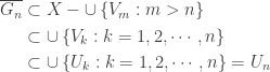
$\displaystyle \begin{aligned} \overline{G_n}&\subset X-\cup \left\{V_m: m > n \right\} \\&\subset \cup \left\{V_k: k=1,2,\cdots,n \right\} \\&\subset \cup \left\{U_k: k=1,2,\cdots,n \right\}=U_n \end{aligned}$

We have just established that $\mathcal{G}$ is a shrinking of $\mathcal{U}$ , or that $\mathcal{U}$ is shrinkable.

For the other direction, to show that $X$ is countably paracompact, we show that the condition in Theorem 4 is satisfied. Let $\left\{A_1,A_2,A_3,\cdots \right\}$ be a decreasing sequence of closed subsets of $X$ with empty intersection. Then $\mathcal{U}=\left\{U_1,U_2,U_3,\cdots \right\}$ be an open cover of $X$ where $U_n=X-A_n$ for each $n$ . By assumption, $\mathcal{U}$ is shrinkable. Let $\mathcal{V}=\left\{V_1,V_2,V_3,\cdots \right\}$ be a shrinking. We can assume that $\mathcal{V}$ is an increasing sequence of open sets.

For each $n$ , let $B_n=X-\overline{V_n}$ . We claim that $\left\{B_1,B_2,B_3,\cdots \right\}$ is a decreasing sequence of open sets that expand the closed sets $A_n$ and that $\bigcap_{n=1}^\infty \overline{B_n}=\varnothing$ . The expansion part follows from the following:

$A_n=X-U_n \subset X-\overline{V_n}=B_n$

The part about decreasing follows from:

$B_{n+1}=X-\overline{V_{n+1}} \subset X-\overline{V_n}=B_n$

We show that $\bigcap_{n=1}^\infty \overline{B_n}=\varnothing$ . To this end, let $x \in X$ . Then $x \in V_n$ for some $n$ . We claim that $x \notin \overline{B_n}$ . Suppose $x \in \overline{B_n}$ . Since $V_n$ is an open set containing $x$ , $V_n$ must contain a point of $B_n$ , say $y$ . Since $y \in B_n$ , $y \notin \overline{V_n}$ . This in turns means that $y \notin V_n$ , a contradiction. Thus we have $x \notin \overline{B_n}$ as claimed. We have established that every point of $X$ is not in $\overline{B_n}$ for some $n$ . Thus the intersection of all the $\overline{B_n}$ must be empty. We have established the condition in Theorem 4 is satisfied. Thus $X$ is countably paracompact. $\square$

Corollary 6
If $X$ is a shrinking space, then $X$ is countably paracompact.

____________________________________________________________________

Reference

Ball, B. J., Countable Paracompactness in Linearly Ordered Spaces, Proc. Amer. Math. Soc., 5, 190-192, 1954. (link)
Rudin, M. E., A Normal Space $X$ for which $X \times I$ is not Normal, Fund. Math., 73, 179-486, 1971. (link)
Rudin, M. E., Dowker Spaces, Handbook of Set-Theoretic Topology (K. Kunen and J. E. Vaughan, eds), Elsevier Science Publishers B. V., Amsterdam, (1984) 761-780.
Wikipedia Entry on Dowker Spaces (link)

____________________________________________________________________
$\copyright \ 2016 \text{ by Dan Ma}$

Counterexample 106 from Steen and Seebach

Posted on August 18, 2015 by Dan Ma

As the title suggests, this post discusses counterexample 106 in the well known book Counterexamples in Topology by Steen and Seebach [2]. We extend the discussion by adding two facts not found in the book.

The counterexample 106 is the space $X=\omega_1 \times I^I$ , which is the product of $\omega_1$ with the interval topology (ordered topology) and the product space $I^I=\prod_{t \in I} I$ where $I$ is of course the unit interval $[0,1]$ . The notation of $\omega_1$ , the first uncountable ordinal, in Steen and Seebach is $[0,\Omega)$ .

Another way to notate the example $X$ is the product space $\prod_{t \in I} X_t$ where $X_0$ is $\omega_1$ and $X_t$ is the unit interval $I$ for all $t>0$ . Thus in this product space, all factors except for one factor is the unit interval and the lone non-compact factor is the first uncountable ordinal. The factor of $\omega_1$ makes this product space an interesting example.

The basic topological properties of the space $X=\omega_1 \times I^I$ that are covered in [2] are:

The space $X$ is Hausdorff and completely regular.
The space $X$ is countably compact.
The space $X$ is neither compact nor sequentially compact.
The space $X$ is neither separable, Lindelof nor $\sigma$ -compact.
The space $X$ is not first countable.
The space $X$ is locally compact.

All the above bullet points are discussed in Steen and Seebach. In this post we add the following two facts.

The space $X$ is not normal.
The space $X$ has a dense subspace that is normal.

It follows from these bullet points that the space $X$ is an example of a completely regular space that is not normal. Not being a normal space, $X$ is then not metrizable. Of course there are other ways to show that $X$ is not metrizable. One is that neither of the two factors $\omega_1$ or $I^I$ is metrizable. Another is that $X$ is not first countable.

The space $X$ is not normal

Now we are ready to discuss the non-normality of the example. It is a natural question to ask whether the example $X=\omega_1 \times I^I$ is normal. The fact that it was not discussed in [2] could be that the tool for answering the normality question was not yet available at the time [2] was originally published, though we do not know for sure. It turns out that the tool became available in the paper [1] published a few years after the publication of [2]. The key to showing the normality (or the lack of) in the example $X=\omega_1 \times I^I$ is to show whether the second factor $I^I$ is a countably tight space.

The tool in [1] is this theorem: for any compact space $Y$ , the product $\omega_1 \times Y$ is normal if and only if $Y$ is countably tight. For a proof of this theorem, see here. Thus the normality of the space $X$ (or the lack of) hinges on whether the compact factor $I^I=\prod_{t \in I} I$ is countably tight.

A space $Y$ is countably tight (or has countable tightness) if for each $S \subset Y$ and for each $x \in \overline{S}$ , there exists some countable $B \subset S$ such that $x \in \overline{B}$ . The definitions of tightness in general and countable tightness in particular are discussed here.

To show that the product space $I^I=\prod_{t \in I} I$ is not countably tight, we define $S$ as follows. For each finite $A \subset I=[0,1]$ , define $f_A: I \rightarrow I$ such that $f_A$ maps $A$ to 1 and maps $I \backslash A$ to 0. Let $S$ be the set of $f_A$ for all possible finite $A \subset I$ . Let $f:I \rightarrow I$ be defined by $f(x)=1$ for all $x \in I$ .

It follows that $f \in \overline{S}$ . We claim that for any countable $B \subset S$ , $f \notin \overline{B}$ . Let $B=\{f_{A_1},f_{A_2}, \cdots \} \subset S$ be countable where each $A_j$ is finite. Then choose $a \in I \backslash \bigcup_{j} A_j$ . Consider the open set $U=\prod_{t \in I} W_t$ where $W_t=I$ for $t \ne a$ and $W_a=(0.5,1]$ . Then $f \in U$ and $U \cap B=\varnothing$ . Thus $f \notin \overline{B}$ . This shows that the product space $I^I=\prod_{t \in I} I$ is not countably tight.

By Theorem 1 found in this link, the space $X=\omega_1 \times I^I$ is not normal.

The space $X$ has a dense subspace that is normal

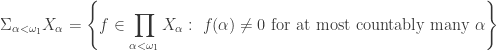
Now that we know $X=\omega_1 \times I^I$ is not normal, a natural question is whether it has a dense subspace that is normal. Consider the subspace $\omega_1 \times S$ where $S$ is the $\Sigma$ -product $S=\Sigma_{t \in I} I$ where $S$ is the space of all $f \in I^I$ such that for each $f$ , $f(x) \ne 0$ for at most countably many $x \in I$ .

The subspace $S$ is dense in the product space $I^I$ . Thus $\omega_1 \times S$ is dense in $X=\omega_1 \times I^I$ . The space $S$ is normal since the $\Sigma$ -product of separable metric spaces is normal (see here). Furthermore, $\omega_1$ can be embedded as a closed subspace of $S=\Sigma_{t \in I} I$ . Then $\omega_1 \times S$ is homeomorphic to a closed subspace of $S \times S$ . Note that $S \times S \cong S$ . Since $\omega_1 \times S$ can be embedded as a closed subspace of the normal space $S$ , the space $\omega_1 \times S$ is normal.

Reference

Nogura, T., Tightness of compact Hausdorff space and normality of product spaces, J. Math. Soc. Japan, 28, 360-362, 1976
Steen, L. A., Seebach, J. A., Counterexamples in Topology, Dover Publications, Inc., New York, 1995.

$\copyright$ 2015 Dan Ma

Revised January 28, 2021

Normality in the powers of countably compact spaces

Posted on May 17, 2015 by Dan Ma

Let $\omega_1$ be the first uncountable ordinal. The topology on $\omega_1$ we are interested in is the ordered topology, the topology induced by the well ordering. The space $\omega_1$ is also called the space of all countable ordinals since it consists of all ordinals that are countable in cardinality. It is a handy example of a countably compact space that is not compact. In this post, we consider normality in the powers of $\omega_1$ . We also make comments on normality in the powers of a countably compact non-compact space.

Let $\omega$ be the first infinite ordinal. It is well known that $\omega^{\omega_1}$ , the product space of $\omega_1$ many copies of $\omega$ , is not normal (a proof can be found in this earlier post). This means that any product space $\prod_{\alpha<\kappa} X_\alpha$ , with uncountably many factors, is not normal as long as each factor $X_\alpha$ contains a countable discrete space as a closed subspace. Thus in order to discuss normality in the product space $\prod_{\alpha<\kappa} X_\alpha$ , the interesting case is when each factor is infinite but contains no countable closed discrete subspace (i.e. no closed copies of $\omega$ ). In other words, the interesting case is that each factor $X_\alpha$ is a countably compact space that is not compact (see this earlier post for a discussion of countably compactness). In particular, we would like to discuss normality in $X^{\kappa}$ where $X$ is a countably non-compact space. In this post we start with the space $X=\omega_1$ of the countable ordinals. We examine $\omega_1$ power $\omega_1^{\omega_1}$ as well as the countable power $\omega_1^{\omega}$ . The former is not normal while the latter is normal. The proof that $\omega_1^{\omega}$ is normal is an application of the normality of $\Sigma$ -product of the real line.

____________________________________________________________________

The uncountable product

Theorem 1
The product space $\prod_{\alpha<\omega_1} \omega_1=\omega_1^{\omega_1}$ is not normal.

Theorem 1 follows from Theorem 2 below. For any space $X$ , a collection $\mathcal{C}$ of subsets of $X$ is said to have the finite intersection property if for any finite $\mathcal{F} \subset \mathcal{C}$ , the intersection $\cap \mathcal{F} \ne \varnothing$ . Such a collection $\mathcal{C}$ is called an f.i.p collection for short. It is well known that a space $X$ is compact if and only collection $\mathcal{C}$ of closed subsets of $X$ satisfying the finite intersection property has non-empty intersection (see Theorem 1 in this earlier post). Thus any non-compact space has an f.i.p. collection of closed sets that have empty intersection.

In the space $X=\omega_1$ , there is an f.i.p. collection of cardinality $\omega_1$ using its linear order. For each $\alpha<\omega_1$ , let $C_\alpha=\left\{\beta<\omega_1: \alpha \le \beta \right\}$ . Let $\mathcal{C}=\left\{C_\alpha: \alpha < \omega_1 \right\}$ . It is a collection of closed subsets of $X=\omega_1$ . It is an f.i.p. collection and has empty intersection. It turns out that for any countably compact space $X$ with an f.i.p. collection of cardinality $\omega_1$ that has empty intersection, the product space $X^{\omega_1}$ is not normal.

Theorem 2
Let $X$ be a countably compact space. Suppose that there exists a collection $\mathcal{C}=\left\{C_\alpha: \alpha < \omega_1 \right\}$ of closed subsets of $X$ such that $\mathcal{C}$ has the finite intersection property and that $\mathcal{C}$ has empty intersection. Then the product space $X^{\omega_1}$ is not normal.

Proof of Theorem 2
Let’s set up some notations on product space that will make the argument easier to follow. By a standard basic open set in the product space $X^{\omega_1}=\prod_{\alpha<\omega_1} X$ , we mean a set of the form $O=\prod_{\alpha<\omega_1} O_\alpha$ such that each $O_\alpha$ is an open subset of $X$ and that $O_\alpha=X$ for all but finitely many $\alpha<\omega_1$ . Given a standard basic open set $O=\prod_{\alpha<\omega_1} O_\alpha$ , the notation $\text{Supp}(O)$ refers to the finite set of $\alpha$ for which $O_\alpha \ne X$ . For any set $M \subset \omega_1$ , the notation $\pi_M$ refers to the projection map from $\prod_{\alpha<\omega_1} X$ to the subproduct $\prod_{\alpha \in M} X$ . Each element $d \in X^{\omega_1}$ can be considered a function $d: \omega_1 \rightarrow X$ . By $(d)_\alpha$ , we mean $(d)_\alpha=d(\alpha)$ .

For each $t \in X$ , let $f_t: \omega_1 \rightarrow X$ be the constant function whose constant value is $t$ . Consider the following subspaces of $X^{\omega_1}$ .

$H=\prod_{\alpha<\omega_1} C_\alpha$

$\displaystyle K=\left\{f_t: t \in X \right\}$

Both $H$ and $K$ are closed subsets of the product space $X^{\omega_1}$ . Because the collection $\mathcal{C}$ has empty intersection, $H \cap K=\varnothing$ . We show that $H$ and $K$ cannot be separated by disjoint open sets. To this end, let $U$ and $V$ be open subsets of $X^{\omega_1}$ such that $H \subset U$ and $K \subset V$ .

Let $d_1 \in H$ . Choose a standard basic open set $O_1$ such that $d_1 \in O_1 \subset U$ . Let $S_1=\text{Supp}(O_1)$ . Since $S_1$ is the support of $O_1$ , it follows that $\pi_{S_1}^{-1}(\pi_{S_1}(d_1)) \subset O_1 \subset U$ . Since $\mathcal{C}$ has the finite intersection property, there exists $a_1 \in \bigcap_{\alpha \in S_1} C_\alpha$ .

Define $d_2 \in H$ such that $(d_2)_\alpha=a_1$ for all $\alpha \in S_1$ and $(d_2)_\alpha=(d_1)_\alpha$ for all $\alpha \in \omega_1-S_1$ . Choose a standard basic open set $O_2$ such that $d_2 \in O_2 \subset U$ . Let $S_2=\text{Supp}(O_2)$ . It is possible to ensure that $S_1 \subset S_2$ by making more factors of $O_2$ different from $X$ . We have $\pi_{S_2}^{-1}(\pi_{S_2}(d_2)) \subset O_2 \subset U$ . Since $\mathcal{C}$ has the finite intersection property, there exists $a_2 \in \bigcap_{\alpha \in S_2} C_\alpha$ .

Now choose a point $d_3 \in H$ such that $(d_3)_\alpha=a_2$ for all $\alpha \in S_2$ and $(d_3)_\alpha=(d_2)_\alpha$ for all $\alpha \in \omega_1-S_2$ . Continue on with this inductive process. When the inductive process is completed, we have the following sequences:

a sequence $d_1,d_2,d_3,\cdots$ of point of $H=\prod_{\alpha<\omega_1} C_\alpha$ ,
a sequence $S_1 \subset S_2 \subset S_3 \subset \cdots$ of finite subsets of $\omega_1$ ,
a sequence $a_1,a_2,a_3,\cdots$ of points of $X$

such that for all $n \ge 2$ , $(d_n)_\alpha=a_{n-1}$ for all $\alpha \in S_{n-1}$ and $\pi_{S_n}^{-1}(\pi_{S_n}(d_n)) \subset U$ . Let $A=\left\{a_1,a_2,a_3,\cdots \right\}$ . Either $A$ is finite or $A$ is infinite. Let’s examine the two cases.

Case 1
Suppose that $A$ is infinite. Since $X$ is countably compact, $A$ has a limit point $a$ . That means that every open set containing $a$ contains some $a_n \ne a$ . For each $n \ge 2$ , define $y_n \in \prod_{\alpha< \omega_1} X$ such that

$(y_n)_\alpha=(d_n)_\alpha=a_{n-1}$ for all $\alpha \in S_n$ ,
$(y_n)_\alpha=a$ for all $\alpha \in \omega_1-S_n$

From the induction step, we have $y_n \in \pi_{S_n}^{-1}(\pi_{S_n}(d_n)) \subset U$ for all $n$ . Let $t=f_a \in K$ , the constant function whose constant value is $a$ . It follows that $t$ is a limit of $\left\{y_1,y_2,y_3,\cdots \right\}$ . This means that $t \in \overline{U}$ . Since $t \in K \subset V$ , $U \cap V \ne \varnothing$ .

Case 2
Suppose that $A$ is finite. Then there is some $m$ such that $a_m=a_j$ for all $j \ge m$ . For each $n \ge 2$ , define $y_n \in \prod_{\alpha< \omega_1} X$ such that

$(y_n)_\alpha=(d_n)_\alpha=a_{n-1}$ for all $\alpha \in S_n$ ,
$(y_n)_\alpha=a_m$ for all $\alpha \in \omega_1-S_n$

As in Case 1, we have $y_n \in \pi_{S_n}^{-1}(\pi_{S_n}(d_n)) \subset U$ for all $n$ . Let $t=f_{a_m} \in K$ , the constant function whose constant value is $a_m$ . It follows that $t=y_n$ for all $n \ge m+1$ . Thus $U \cap V \ne \varnothing$ .

Both cases show that $U \cap V \ne \varnothing$ . This completes the proof the product space $X^{\omega_1}$ is not normal. $\blacksquare$

____________________________________________________________________

The countable product

Theorem 3
The product space $\prod_{\alpha<\omega} \omega_1=\omega_1^{\omega}$ is normal.

Proof of Theorem 3
The proof here actually proves more than normality. It shows that $\prod_{\alpha<\omega} \omega_1=\omega_1^{\omega}$ is collectionwise normal, which is stronger than normality. The proof makes use of the $\Sigma$ -product of $\kappa$ many copies of $\mathbb{R}$ , which is the following subspace of the product space $\mathbb{R}^{\kappa}$ .

$\Sigma(\kappa)=\left\{x \in \mathbb{R}^{\kappa}: x(\alpha) \ne 0 \text{ for at most countably many } \alpha<\kappa \right\}$

It is well known that $\Sigma(\kappa)$ is collectionwise normal (see this earlier post). We show that $\prod_{\alpha<\omega} \omega_1=\omega_1^{\omega}$ is a closed subspace of $\Sigma(\kappa)$ where $\kappa=\omega_1$ . Thus $\omega_1^{\omega}$ is collectionwise normal. This is established in the following claims.

Claim 1
We show that the space $\omega_1$ is embedded as a closed subspace of $\Sigma(\omega_1)$ .

For each $\beta<\omega_1$ , define $f_\beta:\omega_1 \rightarrow \mathbb{R}$ such that $f_\beta(\gamma)=1$ for all $\gamma<\beta$ and $f_\beta(\gamma)=0$ for all $\beta \le \gamma <\omega_1$ . Let $W=\left\{f_\beta: \beta<\omega_1 \right\}$ . We show that $W$ is a closed subset of $\Sigma(\omega_1)$ and $W$ is homeomorphic to $\omega_1$ according to the mapping $f_\beta \rightarrow W$ .

First, we show $W$ is closed by showing that $\Sigma(\omega_1)-W$ is open. Let $y \in \Sigma(\omega_1)-W$ . We show that there is an open set containing $y$ that contains no points of $W$ .

Suppose that for some $\gamma<\omega_1$ , $y_\gamma \in O=\mathbb{R}-\left\{0,1 \right\}$ . Consider the open set $Q=(\prod_{\alpha<\omega_1} Q_\alpha) \cap \Sigma(\omega_1)$ where $Q_\alpha=\mathbb{R}$ except that $Q_\gamma=O$ . Then $y \in Q$ and $Q \cap W=\varnothing$ .

So we can assume that for all $\gamma<\omega_1$ , $y_\gamma \in \left\{0, 1 \right\}$ . There must be some $\theta$ such that $y_\theta=1$ . Otherwise, $y=f_0 \in W$ . Since $y \ne f_\theta$ , there must be some $\delta<\gamma$ such that $y_\delta=0$ . Now choose the open interval $T_\theta=(0.9,1.1)$ and the open interval $T_\delta=(-0.1,0.1)$ . Consider the open set $M=(\prod_{\alpha<\omega_1} M_\alpha) \cap \Sigma(\omega_1)$ such that $M_\alpha=\mathbb{R}$ except for $M_\theta=T_\theta$ and $M_\delta=T_\delta$ . Then $y \in M$ and $M \cap W=\varnothing$ . We have just established that $W$ is closed in $\Sigma(\omega_1)$ .

Consider the mapping $f_\beta \rightarrow W$ . Based on how it is defined, it is straightforward to show that it is a homeomorphism between $\omega_1$ and $W$ .

Claim 2
The $\Sigma$ -product $\Sigma(\omega_1)$ has the interesting property it is homeomorphic to its countable power, i.e.

$\Sigma(\omega_1) \cong \Sigma(\omega_1) \times \Sigma(\omega_1) \times \Sigma(\omega_1) \cdots \ \ \ \ \ \ \ \ \ \ \ \text{(countably many times)}$

Because each element of $\Sigma(\omega_1)$ is nonzero only at countably many coordinates, concatenating countably many elements of $\Sigma(\omega_1)$ produces an element of $\Sigma(\omega_1)$ . Thus Claim 2 can be easily verified. With above claims, we can see that

$\displaystyle \omega_1^{\omega}=\omega_1 \times \omega_1 \times \omega_1 \times \cdots \subset \Sigma(\omega_1) \times \Sigma(\omega_1) \times \Sigma(\omega_1) \cdots \cong \Sigma(\omega_1)$

Thus $\omega_1^{\omega}$ is a closed subspace of $\Sigma(\omega_1)$ . Any closed subspace of a collectionwise normal space is collectionwise normal. We have established that $\omega_1^{\omega}$ is normal. $\blacksquare$

____________________________________________________________________

The normality in the powers of $X$

We have established that $\prod_{\alpha<\omega_1} \omega_1=\omega_1^{\omega_1}$ is not normal. Hence any higher uncountable power of $\omega_1$ is not normal. We have also established that $\prod_{\alpha<\omega} \omega_1=\omega_1^{\omega}$ , the countable power of $\omega_1$ is normal (in fact collectionwise normal). Hence any finite power of $\omega_1$ is normal. However $\omega_1^{\omega}$ is not hereditarily normal. One of the exercises below is to show that $\omega_1 \times \omega_1$ is not hereditarily normal.

Theorem 2 can be generalized as follows:

Theorem 4
Let $X$ be a countably compact space has an f.i.p. collection $\mathcal{C}$ of closed sets such that $\bigcap \mathcal{C}=\varnothing$ . Then $X^{\kappa}$ is not normal where $\kappa=\lvert \mathcal{C} \lvert$ .

The proof of Theorem 2 would go exactly like that of Theorem 2. Consider the following two theorems.

Theorem 5
Let $X$ be a countably compact space that is not compact. Then there exists a cardinal number $\kappa$ such that $X^{\kappa}$ is not normal and $X^{\tau}$ is normal for all cardinal number $\tau<\kappa$ .

By the non-compactness of $X$ , there exists an f.i.p. collection $\mathcal{C}$ of closed subsets of $X$ such that $\bigcap \mathcal{C}=\varnothing$ . Let $\kappa$ be the least cardinality of such an f.i.p. collection. By Theorem 4, that $X^{\kappa}$ is not normal. Because $\kappa$ is least, any smaller power of $X$ must be normal.

Theorem 6
Let $X$ be a space that is not countably compact. Then $X^{\kappa}$ is not normal for any cardinal number $\kappa \ge \omega_1$ .

Since the space $X$ in Theorem 6 is not countably compact, it would contain a closed and discrete subspace that is countable. By a theorem of A. H. Stone, $\omega^{\omega_1}$ is not normal. Then $\omega^{\omega_1}$ is a closed subspace of $X^{\omega_1}$ .

Thus between Theorem 5 and Theorem 6, we can say that for any non-compact space $X$ , $X^{\kappa}$ is not normal for some cardinal number $\kappa$ . The $\kappa$ from either Theorem 5 or Theorem 6 is at least $\omega_1$ . Interestingly for some spaces, the $\kappa$ can be much smaller. For example, for the Sorgenfrey line, $\kappa=2$ . For some spaces (e.g. the Michael line), $\kappa=\omega$ .

Theorems 4, 5 and 6 are related to a theorem that is due to Noble.

Theorem 7 (Noble)
If each power of a space $X$ is normal, then $X$ is compact.

A proof of Noble’s theorem is given in this earlier post, the proof of which is very similar to the proof of Theorem 2 given above. So the above discussion the normality of powers of $X$ is just another way of discussing Theorem 7. According to Theorem 7, if $X$ is not compact, some power of $X$ is not normal.

The material discussed in this post is excellent training ground for topology. Regarding powers of countably compact space and product of countably compact spaces, there are many topics for further discussion/investigation. One possibility is to examine normality in $X^{\kappa}$ for more examples of countably compact non-compact $X$ . One particular interesting example would be a countably compact non-compact $X$ such that the least power $\kappa$ for non-normality in $X^{\kappa}$ is more than $\omega_1$ . A possible candidate could be the second uncountable ordinal $\omega_2$ . By Theorem 2, $\omega_2^{\omega_2}$ is not normal. The issue is whether the $\omega_1$ power $\omega_2^{\omega_1}$ and countable power $\omega_2^{\omega}$ are normal.

____________________________________________________________________

Exercises

Exercise 1
Show that $\omega_1 \times \omega_1$ is not hereditarily normal.

Exercise 2
Show that the mapping $f_\beta \rightarrow W$ in Claim 3 in the proof of Theorem 3 is a homeomorphism.

Exercise 3
The proof of Theorem 3 shows that the space $\omega_1$ is a closed subspace of the $\Sigma$ -product of the real line. Show that $\omega_1$ can be embedded in the $\Sigma$ -product of arbitrary spaces.

For each $\alpha<\omega_1$ , let $X_\alpha$ be a space with at least two points. Let $p \in \prod_{\alpha<\omega_1} X_\alpha$ . The $\Sigma$ -product of the spaces $X_\alpha$ is the following subspace of the product space $\prod_{\alpha<\omega_1} X_\alpha$ .

$\Sigma(X_\alpha)=\left\{x \in \prod_{\alpha<\omega_1} X_\alpha: x(\alpha) \ne p(\alpha) \ \text{for at most countably many } \alpha<\omega_1 \right\}$

The point $p$ is the center of the $\Sigma$ -product. Show that the space $\Sigma(X_\alpha)$ contains $\omega_1$ as a closed subspace.

Exercise 4
Find a direct proof of Theorem 3, that $\omega_1^{\omega}$ is normal.

____________________________________________________________________
$\copyright \ 2015 \text{ by Dan Ma}$

The product of uncountably many factors is never hereditarily normal

Posted on May 3, 2015 by Dan Ma

The space $Y=\prod_{\alpha<\omega_1} \left\{0,1 \right\}=\left\{0,1 \right\}^{\omega_1}$ is the product of $\omega_1$ many copies of the two-element set $\left\{0,1 \right\}$ where $\omega_1$ is the first uncountable ordinal. It is a compact space by Tychonoff’s theorem. It is a normal space since every compact Hausdorff space is normal. A space is hereditarily normal if every subspace is normal. Is the space $Y$ hereditarily normal? In this post, we give two proofs that it is not hereditarily normal. It then follows that any product space $\prod X_\alpha$ cannot be hereditarily normal as long as there are uncountably many factors and every factor has at least two point.

____________________________________________________________________

The connection with a theorem of Katetov

It turns out that there is a connection with a theorem of Katetov. For any compact space, knowing hereditary normality of the first several self product spaces can reveal a great deal of information about the compact space. More specifically, for any compact space $X$ , knowing whether $X$ , $X^2$ and $X^3$ are hereditarily normal can tell us whether $X$ is metrizable. If all three are hereditarily normal, then $X$ is metrizable. If one of the three self products is not hereditarily normal, then $X$ is not metrizable. This fact is based on a theorem of Katetov (see this previous post). The space $Y=\left\{0,1 \right\}^{\omega_1}$ is not metrizable since it is not first countable (see Problem 1 below). Thus one of its first three self products must fail to be hereditarily normal.

These two proofs are not direct proof in the sense that a non-normal subspace is not explicitly produced. Instead the proofs use other theorem or basic but important background results. One of the two proofs (#2) uses a theorem of Katetov on hereditarily normal spaces. The other proof (#1) uses the fact that the product of uncountably many copies of a countable discrete space is not normal. We believe that these two proofs and the required basic facts are an important training ground for topology. We list out these basic facts as exercises. Anyone who wishes to fill in the gaps can do so either by studying the links provided or by consulting other sources.

The theorem of Katetov mentioned earlier provides a great exercise – for any non-metrizable compact space $X$ , determine where the hereditary normality fails. Does it fail in $X$ , $X^2$ or $X^3$ ? This previous post examines a small list of compact non-metrizable spaces. In all the examples in this list, the hereditary normality fails in $X$ or $X^2$ . The space $Y=\left\{0,1 \right\}^{\omega_1}$ can be added to this list. All the examples in this list are defined using no additional set theory axioms beyond ZFC. A natural question: does there exist an example of compact non-metrizable space $X$ such that the hereditary normality holds in $X^2$ and fails in $X^3$ ? It turns out that this was a hard problem and the answer is independent of ZFC. This previous post provides a brief discussion and has references for the problem.

All spaces under consideration are Hausdorff spaces.

____________________________________________________________________

Exercises

Problem 1
Let $X$ be a compact space. Show that $X$ is normal.

Problem 2
For each $\alpha<\omega_1$ , let $A_\alpha$ be a set with cardinality $\le \omega_1$ . Show that $\lvert \bigcup_{\alpha<\omega_1} A_\alpha \lvert \le \omega_1$ .

Problem 2 holds for any infinite cardinal, not just $\omega_1$ . One reference for Problem 2 is Lemma 10.21 on page 30 of Set Theorey, An Introduction to Independence Proofs by Kenneth Kunen.

Problem 3
For each $\alpha<\omega_1$ , let $X_\alpha$ be a space with at least two points. Show that for every point $p \in \prod_{\alpha<\omega_1} X_\alpha$ , there does not exist a countable base at the point $p$ . In other words, the product space $\prod_{\alpha<\omega_1} X_\alpha$ is not first countable at every point. It follows that product space $\prod_{\alpha<\omega_1} X_\alpha$ is not metrizable.

Problem 4
In any space, a $G_\delta$ -set is a set that is the intersection of countably many open sets. When a singleton set $\left\{ x \right\}$ is a $G_\delta$ -set, we say the point $x$ is a $G_\delta$ -point. For each $\alpha<\omega_1$ , let $X_\alpha$ be a space with at least two points. Show that every point $p$ in the product space $\prod_{\alpha<\omega_1} X_\alpha$ is not a $G_\delta$ -point.

Note that Problem 4 implies Problem 3.

For Problem 3 and Problem 4, use the fact that there are uncountably many factors and that a basic open set in the product space is of the form $\prod_{\alpha<\omega_1} O_\alpha$ and that it has only finitely many coordinates at which $O_\alpha \ne X_\alpha$ .

Problem 5
For each $\alpha<\omega_1$ , let $X_\alpha=\left\{0,1,2,\cdots \right\}$ be the set of non-negative integers with the discrete topology. Show that the product space $\prod_{\alpha<\omega_1} X_\alpha$ is not normal.

See here for a discussion of Problem 5.

Problem 6
Let $\displaystyle Y=\left\{0,1 \right\}^{\omega_1}$ . Show that $Y$ has a countably infinite subspace

$W=\left\{y_0,y_1,y_2,y_3\cdots \right\}$

such that $W$ is relatively discrete. In other words, $W$ is discrete in the subspace topology of $W$ . However $W$ is not discrete in the product space $Y$ since $Y$ is compact.

____________________________________________________________________

Proof #1

Let $\displaystyle Y=\left\{0,1 \right\}^{\omega_1}$ . We show that $Y$ is not hereditarily normal.

Note that the product space $\displaystyle Y=\left\{0,1 \right\}^{\omega_1}$ can be written as the product of $\omega_1$ many copies of itself:

$\displaystyle \left\{0,1 \right\}^{\omega_1} \cong \left\{0,1 \right\}^{\omega_1} \times \left\{0,1 \right\}^{\omega_1} \times \left\{0,1 \right\}^{\omega_1} \times \cdots \ \ \ \ \ \ \ \ \ \ \ \ \ \ \ \ \ \ \ \ \ (1)$

The fact (1) follows from the fact that the union of $\omega_1$ many pairwise disjoint sets, each of which has cardinality $\omega_1$ , has cardinality $\omega_1$ (see Problem 2). The space $\left\{0,1 \right\}^{\omega_1}$ has a countably infinite subspace that is relatively discrete (see Problem 6). In other words, it has a subspace that is homemorphic to $\omega=\left\{0,1,2,\cdots \right\}$ where $\omega$ has the discrete topology. Thus the following is homeomorphic to a subspace of $\displaystyle Y=\left\{0,1 \right\}^{\omega_1}$ .

$\displaystyle \omega^{\omega_1} = \omega \times \omega \times \omega \times \cdots \ \ \ \ \ \ \ \ \ \ \ \ \ \ \ \ \ \ \ \ \ \ \ \ \ \ \ \ \ \ \ \ \ \ \ \ \ \ \ \ \ \ \ \ \ \ \ \ \ \ \ (2)$

By Problem 5, the space $\omega^{\omega_1}$ is not normal. Hence the compact space $\displaystyle Y=\left\{0,1 \right\}^{\omega_1}$ contains the non-normal space $\omega^{\omega_1}$ and is thus not hereditarily normal. $\blacksquare$

____________________________________________________________________

Proof #2

Let $\displaystyle Y=\left\{0,1 \right\}^{\omega_1}$ . We show that $Y$ is not hereditarily normal. This proof uses a theorem of Katetov, discussed in this previous post and stated below.

Theorem 1
If $X_1 \times X_2$ is hereditarily normal (i.e. every one of its subspaces is normal), then one of the following condition holds:

The factor $X_1$ is perfectly normal.
Every countable and infinite subset of the factor $X_2$ is closed.

First, $Y$ can be written as the product of two copies of itself:

$\displaystyle \left\{0,1 \right\}^{\omega_1} \cong \left\{0,1 \right\}^{\omega_1} \times \left\{0,1 \right\}^{\omega_1} \ \ \ \ \ \ \ \ \ \ \ \ \ \ \ \ \ \ \ \ \ \ \ \ \ \ \ \ \ \ \ \ \ \ \ \ \ \ \ \ \ \ \ (3)$

This is because the union of two disjoints sets, each of which has cardinality $\omega_1$ , has carinality $\omega_1$ . Note that the countably infinite subset $W$ from Problem 6 is not a closed subset of $Y$ . If it were, the compact space $Y$ would contain an infinite set with no limit point. Thus the second condition of Theorem 1 is not satisfied. If $Y \cong Y \times Y$ were to be hereditarily normal, then the first condition must be satisfied, i.e. $Y$ is perfectly normal (meaning that $Y$ is normal and that every closed subset of it is a $G_\delta$ -set). However, Problem 4 indicates that no point in $Y$ can be a $G_\delta$ point. Therefore $Y$ cannot be hereditarily normal. $\blacksquare$

____________________________________________________________________

Corollary

The product of uncountably many spaces, each one of which has at least two points, contains a homeomorphic copy of the space $\displaystyle Y=\left\{0,1 \right\}^{\omega_1}$ . Thus such a product space can never be hereditarily normal. We state this more formally below.

Theorem 2
Let $\kappa$ be any uncountable cardinal. For each $\alpha<\kappa$ , let $X_\alpha$ be a space with at least two points. Then $\prod_{\alpha<\kappa} X_\alpha$ is not hereditarily normal.

____________________________________________________________________
$\copyright \ 2015 \text{ by Dan Ma}$

The Sorgenfrey plane is subnormal

Posted on May 7, 2014 by Dan Ma

The Sorgenfrey line is the real line with the topology generated by the base of half-open intervals of the form $[a,b)$ . The Sorgenfrey line is one of the most important counterexamples in general topology. One of the often recited facts about this counterexample is that the Sorgenfrey plane (the square of the Sorgengfrey line) is not normal. We show that, though far from normal, the Sorgenfrey plane is subnormal.

A subset $M$ of a space $Y$ is a $G_\delta$ subset of $Y$ (or a $G_\delta$ -set in $Y$ ) if $M$ is the intersection of countably many open subsets of $Y$ . A subset $M$ of a space $Y$ is a $F_\sigma$ subset of $Y$ (or a $F_\sigma$ -set in $Y$ ) if $Y-M$ is a $G_\delta$ -set in $Y$ (equivalently if $M$ is the union of countably many closed subsets of $Y$ ).

A space $Y$ is normal if for any disjoint closed subsets $H$ and $K$ of $Y$ , there exist disjoint open subsets $U_H$ and $U_K$ of $Y$ such that $H \subset U_H$ and $K \subset U_K$ . A space $Y$ is subnormal if for any disjoint closed subsets $H$ and $K$ of $Y$ , there exist disjoint $G_\delta$ subsets $V_H$ and $V_K$ of $Y$ such that $H \subset V_H$ and $K \subset V_K$ . Clearly any normal space is subnormal. The Sorgenfrey plane is an example of a subnormal space that is not normal.

In the proof of the non-normality of the Sorgenfrey plane in this previous post, one of the two disjoint closed subsets of the Sorgenfrey plane that cannot be separated by disjoint open sets is countable. Thus the Sorgenfrey plane is not only not normal; it is not pseudonormal (also discussed in this previous post). A space $Y$ is pseudonormal if for any disjoint closed subsets $H$ and $K$ of $Y$ (one of which is countable), there exist disjoint open subsets $U_H$ and $U_K$ of $Y$ such that $H \subset U_H$ and $K \subset U_K$ . The examples of the Sorgenfrey plane and $\omega_1 \times (\omega_1+1)$ show that these two weak forms of normality (pseudonormal and subnormal) are not equivalent. The space $\omega_1 \times (\omega_1+1)$ is pseudonormal but not subnormal (see this previous post for the non-subnormality).

A space $Y$ is said to be a perfect space if every closed subset of $Y$ is a $G_\delta$ subset of $Y$ (equivalently, every open subset of $Y$ is an $F_\sigma$ -subset of $Y$ ). It is clear that any perfect space is subnormal. We show that the Sorgenfrey plane is perfect. There are subnormal spaces that are not perfect (see the example below).

____________________________________________________________________

The Sorgenfrey plane is perfect

Let $S$ denote the Sorgenfrey line, i.e., the real line $\mathbb{R}$ topologized using the base of half-open intervals of the form $[a,b)=\left\{x \in \mathbb{R}: a \le x <b \right\}$ . The Sorgenfrey plane is the product space $S \times S$ . We show the following:

Proposition 1
The Sorgenfrey line $S$ is perfect.

Proof of Proposition 1
Let $U$ be a non-empty subset of $S$ . We show that $U$ is a $F_\sigma$ -set. Let $U_0$ be the interior of $U$ in the usual topology. In other words, $U_0$ is the following set:

$U_0=\left\{x \in U: \exists \ (a,b) \text{ such that } x \in (a,b) \text{ and } (a,b) \subset U \right\}$

The real line with the usual topology is perfect. Thus $U_0=\bigcup_{n=1}^\infty F_n$ where each $F_n$ is a closed subset of the real line $\mathbb{R}$ . Since the Sorgenfrey topology is finer than the usual topology, each $F_n$ is also closed in the Sorgenfrey line.

Consider $Y=U-U_0$ . We claim that $Y$ is countable. Suppose $Y$ is uncountable. Since the Sorgenfrey line is hereditarily Lindelof, there exists $y \in Y$ such that $y$ is a limit point of $Y$ (see Corollary 2 in this previous post). Since $y \in Y \subset U$ , $[y,t) \subset U$ for some $t$ . Note that $(y,t) \subset U_0$ , which means that no point of the open interval $(y,t)$ can belong to $Y$ . On the other hand, since $y$ is a limit point of $Y$ , $y<w<t$ for some $w \in Y$ , a contradiction. Thus $Y$ must be countable. It follows that $U$ is the union of countably many closed subsets of $S$ . $\blacksquare$

Proposition 2
If $X$ is perfect and $Y$ is metrizable, then $X \times Y$ is perfect.

Proof of Proposition 2
Let $X$ be perfect. Let $Y$ be a space with a base $\mathcal{B}=\bigcup_{n=1}^\infty \mathcal{B}_n$ such that each $\mathcal{B}_n$ , in addition to being a collection of basic open sets, is a discrete collection. The existence of such a base is equivalent to metrizability, a well known result called Bing’s metrization theorem (see Theorem 4.4.8 in [1]). Let $U$ be a non-empty open subset of $X \times Y$ . We show that it is an $F_\sigma$ -set in $X \times Y$ . For each $x \in U$ , there is some open subset $V$ of $X$ and there is some $W \in \mathcal{B}$ such that $x \in V \times W$ and $V \times \overline{W} \subset U$ . Thus $U$ is the union of a collection of sets of the form $V \times \overline{W}$ . Thus we have:

$U=\bigcup \mathcal{O} \text{ where } \mathcal{O}=\left\{ V_\alpha \times \overline{W_\alpha}: \alpha \in A \right\}$

for some index set $A$ . For each positive integer $m$ , let $\mathcal{O}_m$ be defined by

$\mathcal{O}_m=\left\{V_\alpha \times \overline{W_\alpha} \in \mathcal{O}: W_\alpha \in \mathcal{B}_m \right\}$

For each $\alpha \in A$ , let $V_\alpha=\bigcup_{n=1}^\infty V_{\alpha,n}$ where each $V_{\alpha,n}$ is a closed subset of $X$ . For each pair of positive integers $n$ and $m$ , define $\mathcal{O}_{n,m}$ by

$\mathcal{O}_{n,m}=\left\{V_{\alpha,n} \times \overline{W_\alpha}: V_\alpha \times \overline{W_\alpha} \in \mathcal{O}_m \right\}$

We claim that each $\mathcal{O}_{n,m}$ is a discrete collection of sets in the space $X \times Y$ . Let $(a,b) \in X \times Y$ . Since $\mathcal{B}_m$ is discrete, there exists some open subset $H_b$ of $Y$ with $b \in H_b$ such that $H_b$ can intersect at most one $\overline{W}$ where $W \in \mathcal{B}_m$ . Then $X \times H_b$ is an open subset of $X \times Y$ with $(a,b) \in X \times H_b$ such that $X \times H_b$ can intersect at most one set of the form $V_{\alpha,n} \times \overline{W_\alpha}$ . Then $C_{n,m}=\bigcup \mathcal{O}_{n,m}$ is a closed subset of $X \times Y$ . It is clear that $U$ is the union of $C_{n,m}$ over all countably many possible pairs $n,m$ . Thus $U$ is an $F_\sigma$ -set in $X \times Y$ . $\blacksquare$

Proposition 3
The Sorgenfrey plane $S \times S$ is perfect.

Proof of Proposition 3
To get ready for the proof, consider the product spaces $X_1=\mathbb{R} \times S$ and $X_2=S \times \mathbb{R}$ where $\mathbb{R}$ has the usual topology. By both Proposition 1 and Proposition 2, both $X_1$ and $X_2$ are perfect. Also note that the Sorgenfrey plane topology is finer than the topologies for both $X_1$ and $X_2$ . Thus a closed set in $X_1$ (in $X_2$ ) is also a closed set in $S \times S$ . It follows that any $F_\sigma$ -set in $X_1$ (in $X_2$ ) is also an $F_\sigma$ -set in $S \times S$ .

Let $U$ be a non-empty subset of $S \times S$ . We show that $U$ is a $F_\sigma$ -set. We assume that $U$ is the union of basic open sets of the form $[a,b) \times [a,b)$ . Consider the sets $U_1$ and $U_2$ defined by:

$U_1=\left\{x \in U: \exists \ (a,b) \times [a,b) \text{ such that } x \in (a,b) \times [a,b) \text{ and } (a,b) \times [a,b) \subset U \right\}$

$U_2=\left\{x \in U: \exists \ [a,b) \times (a,b) \text{ such that } x \in [a,b) \times (a,b) \text{ and } [a,b) \times (a,b) \subset U \right\}$

Note that $U_1$ is the interior of $U$ when $U$ is considered as a subspace of $X_1$ . Likewise, $U_2$ is the interior of $U$ when $U$ is considered as a subspace of $X_2$ . Since both $X_1$ and $X_2$ are perfect, $U_1$ and $U_2$ are $F_\sigma$ in $X_1$ and $X_2$ , respectively. Hence both $U_1$ and $U_2$ are $F_\sigma$ -sets in $S \times S$ .

Let $Y=U-(U_1 \cup U_2)$ . We claim that $Y$ is an $F_\sigma$ -set in $S \times S$ . Proposition 3 is established when this claim is proved. To get ready to prove this claim, for each $x=(x_1,x_2) \in S \times S$ , and for each positive integer $k$ , let $B_k(x)$ be the half-open square $B_k(x)=[x_1,x_1+\frac{1}{k}) \times [x_2,x_2+\frac{1}{k})$ . Then $\mathcal{B}(x)=\left\{B_k(x): k=1,2,3,\cdots \right\}$ is a local base at the point $x$ . For each positive integer $k$ , define $Y_k$ by

$Y_k=\left\{y=(y_1,y_2) \in Y: B_k(y) \subset U \right\}$

Clearly $Y=\bigcup_{k=1}^\infty Y_k$ . We claim that each $Y_k$ is closed in $S \times S$ . Suppose $x=(x_1,x_2) \in S \times S-Y_k$ . In relation to the point $x$ , $Y_k$ can be broken into several subsets as follows:

$Y_{k,1}=\left\{y=(y_1,y_2) \in Y_k: y_1=x_1 \text{ and } y_2 \ne x_2 \right\}$

$Y_{k,2}=\left\{y=(y_1,y_2) \in Y_k: y_1 \ne x_1 \text{ and } y_2 = x_2 \right\}$

$Y_{k,\varnothing}=\left\{y=(y_1,y_2) \in Y_k: y_1 \ne x_1 \text{ and } y_2 \ne x_2 \right\}$

Since $x \notin Y_k$ , it follows that $Y_k=Y_{k,1} \cup Y_{k,2} \cup Y_{k,\varnothing}$ . We show that for each of these three sets, there is an open set containing the point $x$ that is disjoint from the set.

Consider $Y_{k,1}$ . If $B_k(x)=[x_1,x_1+\frac{1}{k}) \times [x_2,x_2+\frac{1}{k})$ is disjoint from $Y_{k,1}$ , then we are done. So assume $B_k(x) \cap Y_{k,1} \ne \varnothing$ . Let $t=(t_1,t_2) \in B_k(x) \cap Y_{k,1}$ . Note that $t_1=x_1$ and $t_2 > x_2$ . Now consider the following open set:

$G=B_k(x) \cap \left\{y=(y_1,y_2) \in S \times S: y_2<t_2 \right\}$

The set $G$ is an open set containing the point $x$ . We claim that $G \cap Y_{k,1}=\varnothing$ . Suppose $g \in G \cap Y_{k,1}$ . Then $g_1=x_1$ and $x_2<g_2<t_2$ . Consider the following set:

$H=B_k(g) \cap \left\{h=(h_1,h_2) \in S \times S: g_2<h_2 \right\}$

Note that $H$ is an open subset of $X_2=S \times \mathbb{R}$ . Since $g \in Y_k$ , it follows that $H \subset B_k(g) \subset U$ . Thus $H$ is a subset of the interior of $U$ (as a subspace of $X_2$ ). We have $H \subset U_2$ . It follows that $t \in H$ since

$x_1=g_1=t_1$

$x_2<g_2<t_2<x_2+\frac{1}{k}<g_2+\frac{1}{k}$

On the other hand, $t \in Y_{k,1} \subset Y_k \subset Y$ . Hence $t \notin U_2$ , a contradiction. Thus the claim that $G \cap Y_{k,1}=\varnothing$ must be true.

The case $Y_{k,2}$ is symmetrical to the case $Y_{k,1}$ . Thus by applying a similar argument, there is an open set containing the point $x$ that is disjoint from the set $Y_{k,2}$ .

Now consider the case $Y_{k,\varnothing}$ . If $B_k(x)=[x_1,x_1+\frac{1}{k}) \times [x_2,x_2+\frac{1}{k})$ is disjoint from $Y_{k,\varnothing}$ , then we are done. So assume $B_k(x) \cap Y_{k,\varnothing} \ne \varnothing$ . Let $t=(t_1,t_2) \in B_k(x) \cap Y_{k,\varnothing}$ . Note that $t_1>x_1$ and $t_2 > x_2$ . Now consider the following open set:

$G=B_k(x) \cap \left\{y=(y_1,y_2) \in S \times S: y_1<t_1 \text{ and }y_2<t_2 \right\}$

The set $G$ is an open set containing the point $x$ . We claim that $G \cap Y_{k,\varnothing}=\varnothing$ . Suppose $g \in G \cap Y_{k,\varnothing}$ . Then $x_1<g_1<t_1$ and $x_2<g_2<t_2$ . Consider the following set:

$H=B_k(g) \cap \left\{h=(h_1,h_2) \in S \times S: g_2<h_2 \right\}$

As in the previous case, $H$ is an open subset of $X_2=S \times \mathbb{R}$ . Since $g \in Y_k$ , it follows that $H \subset B_k(g) \subset U$ . As before, $H \subset U_2$ . We also have a contradiction in that $t \in H$ (based on the following)

$x_1<g_1<t_1<x_1+\frac{1}{k}<g_1+\frac{1}{k}$

$x_2<g_2<t_2<x_2+\frac{1}{k}<g_2+\frac{1}{k}$

and on the one hand and $t \in Y_{k,\varnothing} \subset Y=U-(U_1 \cup U_2)$ . Thus the claim that $G \cap Y_{k,\varnothing}=\varnothing$ is true. Take the intersection of the three open sets from the three cases, we have an open set containing $x$ that is disjoint from $Y_k$ . Thus $Y_k$ is closed in $S \times S$ and $Y=\bigcup_{k=1}^\infty Y_k$ is $F_\sigma$ in $S \times S$ . $\blacksquare$

Remarks
The authors of [2] showed that any finite power of the Sorgenfrey line is perfect. The proof in [2] is an inductive proof: if $S^n$ is perfect, then $S^{n+1}$ is perfect. We take the inductive proof in [2] and adapt it for the Sorgenfrey plane. The authors in [2] also proved that for a sequence of spaces $X_1,X_2,X_3,\cdots$ such that the product of any finite number of these spaces is perfect, the product $\prod_{n=1}^\infty X_n$ is perfect. Then $S^\omega$ is perfect.

____________________________________________________________________

A non-perfect example

Any perfect space is subnormal. Subnormal spaces do not have to be perfect. In fact subnormal non-normal spaces do not have to be perfect. From a perfect space that is not normal (e.g. the Sorgenfrey plane), one can generate a subnormal and non-normal space that is not perfect. Let $X$ be a subnormal and non-normal space. Let $Y$ be a normal space that is not perfectly normal. There are many possible choices for $Y$ . If a specific example is needed, one can take $Y=\omega_1$ with the order topology. Let $X \bigoplus Y$ be the disjoint sum (union) of $X$ and $Y$ . The presence of $Y$ destroys the perfectness. It is clear that any two disjoint closed sets can be separated by disjoint $G_\delta$ -sets.

____________________________________________________________________

Reference

Engelking, R., General Topology, Revised and Completed edition, Heldermann Verlag, Berlin, 1989.
Heath, R. W., Michael, E., A property of the Sorgenfrey line, Compositio Math., 23, 185-188, 1971.

____________________________________________________________________
$\copyright \ 2014 \text{ by Dan Ma}$

Dan Ma's Topology Blog

Expository Articles In General Topology

Tag Archives: Non-normal product

Revisiting example 106 from Steen and Seebach

Michael line and Morita’s conjectures

Three conjectures of K Morita

Extracting more information from Dowker’s theorem

kappa-Dowker space and the first conjecture of Morita

Countably paracompact spaces

Counterexample 106 from Steen and Seebach

Normality in the powers of countably compact spaces

The product of uncountably many factors is never hereditarily normal

The Sorgenfrey plane is subnormal