Let  be the first uncountable ordinal. The topology on we are interested in is the ordered topology, the topology induced by the well ordering. The space is also called the space of all countable ordinals since it consists of all ordinals that are countable in cardinality. It is a handy example of a countably compact space that is not compact. In this post, we consider normality in the powers of . We also make comments on normality in the powers of a countably compact non-compact space.
Let  be the first infinite ordinal. It is well known that
  , the product space of many copies of , is not normal (a proof can be found in this earlier post). This means that any product space
  , with uncountably many factors, is not normal as long as each factor
  contains a countable discrete space as a closed subspace. Thus in order to discuss normality in the product space , the interesting case is when each factor is infinite but contains no countable closed discrete subspace (i.e. no closed copies of ). In other words, the interesting case is that each factor is a countably compact space that is not compact (see this earlier post for a discussion of countably compactness). In particular, we would like to discuss normality in
  where
where  is a countably non-compact space. In this post we start with the space
  of the countable ordinals. We examine power
  as well as the countable power
  . The former is not normal while the latter is normal. The proof that is normal is an application of the normality of
  -product of the real line.
____________________________________________________________________
The uncountable product
Theorem 1
The product space  is not normal.
Theorem 1 follows from Theorem 2 below. For any space , a collection  of subsets of is said to have the finite intersection property if for any finite
  , the intersection
  . Such a collection is called an f.i.p collection for short. It is well known that a space is compact if and only collection of closed subsets of satisfying the finite intersection property has non-empty intersection (see Theorem 1 in this earlier post). Thus any non-compact space has an f.i.p. collection of closed sets that have empty intersection.
In the space , there is an f.i.p. collection of cardinality using its linear order. For each  , let
, let  . Let
. Let  . It is a collection of closed subsets of . It is an f.i.p. collection and has empty intersection. It turns out that for any countably compact space with an f.i.p. collection of cardinality that has empty intersection, the product space
  is not normal.
Theorem 2
Let be a countably compact space. Suppose that there exists a collection of closed subsets of such that has the finite intersection property and that has empty intersection. Then the product space is not normal.
Proof of Theorem 2
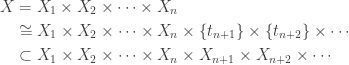
Let’s set up some notations on product space that will make the argument easier to follow. By a standard basic open set in the product space  , we mean a set of the form
  such that each
  is an open subset of and that
  for all but finitely many . Given a standard basic open set , the notation
  refers to the finite set of
  for which
  . For any set
  , the notation
  refers to the projection map from
  to the subproduct
  . Each element
  can be considered a function
  . By
. By  , we mean
  .
.
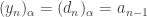
For each  , let
, let  be the constant function whose constant value is
  . Consider the following subspaces of .
Both  and
and  are closed subsets of the product space . Because the collection has empty intersection,
  . We show that and cannot be separated by disjoint open sets. To this end, let
  and
and  be open subsets of such that
  and
and  .
.
Let  . Choose a standard basic open set
  such that
  . Let
. Let  . Since
  is the support of , it follows that
  . Since has the finite intersection property, there exists
  .
.
Define  such that
  for all
  and
and  for all
  . Choose a standard basic open set
  such that
  . Let
. Let  . It is possible to ensure that
  by making more factors of different from . We have
  . Since has the finite intersection property, there exists
  .
.
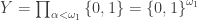
Now choose a point  such that
  for all
  and
and  for all
  . Continue on with this inductive process. When the inductive process is completed, we have the following sequences:
- a sequence
 of point of
  ,
,
- a sequence
 of finite subsets of ,
- a sequence
 of points of
such that for all  ,
,  for all
  and
and  . Let
. Let  . Either
  is finite or is infinite. Let’s examine the two cases.
Case 1
Suppose that is infinite. Since is countably compact, has a limit point  . That means that every open set containing contains some
  . For each , define
  such that
From the induction step, we have  for all
  . Let
. Let  , the constant function whose constant value is . It follows that is a limit of
  . This means that
  . Since
  ,
,  .
.
Case 2
Suppose that is finite. Then there is some  such that
  for all
  . For each , define such that
As in Case 1, we have for all . Let  , the constant function whose constant value is
  . It follows that
  for all
  . Thus .
Both cases show that . This completes the proof the product space is not normal. 
____________________________________________________________________
The countable product
Theorem 3
The product space  is normal.
Proof of Theorem 3
The proof here actually proves more than normality. It shows that is collectionwise normal, which is stronger than normality. The proof makes use of the -product of  many copies of
  , which is the following subspace of the product space
  .
.
It is well known that  is collectionwise normal (see this earlier post). We show that is a closed subspace of where
  . Thus is collectionwise normal. This is established in the following claims.
Claim 1
We show that the space is embedded as a closed subspace of  .
.
For each  , define
  such that
  for all
  and
and  for all
  . Let
. Let  . We show that
  is a closed subset of and is homeomorphic to according to the mapping
  .
.
First, we show is closed by showing that  is open. Let
  . We show that there is an open set containing
  that contains no points of .
Suppose that for some  ,
,  . Consider the open set
  where
where  except that
  . Then
  and
and  .
.
So we can assume that for all ,  . There must be some
  such that
  . Otherwise,
  . Since
  , there must be some
  such that
  . Now choose the open interval
  and the open interval
  . Consider the open set
  such that
  except for
  and
and  . Then
  and
and  . We have just established that is closed in .
Consider the mapping . Based on how it is defined, it is straightforward to show that it is a homeomorphism between and .
Claim 2
The -product has the interesting property it is homeomorphic to its countable power, i.e.
 .
.
Because each element of is nonzero only at countably many coordinates, concatenating countably many elements of produces an element of . Thus Claim 2 can be easily verified. With above claims, we can see that
Thus is a closed subspace of . Any closed subspace of a collectionwise normal space is collectionwise normal. We have established that is normal.
____________________________________________________________________
The normality in the powers of
We have established that is not normal. Hence any higher uncountable power of is not normal. We have also established that , the countable power of is normal (in fact collectionwise normal). Hence any finite power of is normal. However is not hereditarily normal. One of the exercises below is to show that  is not hereditarily normal.
Theorem 2 can be generalized as follows:
Theorem 4
Let be a countably compact space has an f.i.p. collection of closed sets such that  . Then is not normal where
  .
.
The proof of Theorem 2 would go exactly like that of Theorem 2. Consider the following two theorems.
Theorem 5
Let be a countably compact space that is not compact. Then there exists a cardinal number such that is not normal and  is normal for all cardinal number
  .
.
By the non-compactness of , there exists an f.i.p. collection of closed subsets of such that . Let be the least cardinality of such an f.i.p. collection. By Theorem 4, that is not normal. Because is least, any smaller power of must be normal.
Theorem 6
Let be a space that is not countably compact. Then is not normal for any cardinal number  .
.
Since the space in Theorem 6 is not countably compact, it would contain a closed and discrete subspace that is countable. By a theorem of A. H. Stone, is not normal. Then is a closed subspace of .
Thus between Theorem 5 and Theorem 6, we can say that for any non-compact space , is not normal for some cardinal number . The from either Theorem 5 or Theorem 6 is at least . Interestingly for some spaces, the can be much smaller. For example, for the Sorgenfrey line,  . For some spaces (e.g. the Michael line),
  .
.
Theorems 4, 5 and 6 are related to a theorem that is due to Noble.
Theorem 7 (Noble)
If each power of a space is normal, then is compact.
A proof of Noble’s theorem is given in this earlier post, the proof of which is very similar to the proof of Theorem 2 given above. So the above discussion the normality of powers of is just another way of discussing Theorem 7. According to Theorem 7, if is not compact, some power of is not normal.
The material discussed in this post is excellent training ground for topology. Regarding powers of countably compact space and product of countably compact spaces, there are many topics for further discussion/investigation. One possibility is to examine normality in for more examples of countably compact non-compact . One particular interesting example would be a countably compact non-compact such that the least power for non-normality in is more than . A possible candidate could be the second uncountable ordinal  . By Theorem 2,
  is not normal. The issue is whether the power
  and countable power
  are normal.
____________________________________________________________________
Exercises
Exercise 1
Show that is not hereditarily normal.
Exercise 2
Show that the mapping in Claim 3 in the proof of Theorem 3 is a homeomorphism.
Exercise 3
The proof of Theorem 3 shows that the space is a closed subspace of the -product of the real line. Show that can be embedded in the -product of arbitrary spaces.
For each , let be a space with at least two points. Let  . The -product of the spaces is the following subspace of the product space
  .
.
The point  is the center of the -product. Show that the space
  contains as a closed subspace.
Exercise 4
Find a direct proof of Theorem 3, that is normal.
____________________________________________________________________


-compact spaces


 with the ordered topology
 of the square
  is called the diagonal of the space
  -diagonal if
  is a
is a  , i.e.
  , there is an open subset
  and
and  with the order topology. Using interval notion,
 ![X=[0,\omega_1]](https://s0.wp.com/latex.php?latex=X%3D%5B0%2C%5Comega_1%5D&bg=ffffff&fg=333333&s=0&c=20201002) . This is the space of all countable ordinals
. This is the space of all countable ordinals  . Note that any open set of the form
 ![(\alpha, \omega_1] \times (\alpha, \omega_1]](https://s0.wp.com/latex.php?latex=%28%5Calpha%2C+%5Comega_1%5D+%5Ctimes+%28%5Calpha%2C+%5Comega_1%5D&bg=ffffff&fg=333333&s=0&c=20201002) contains the point
contains the point  and contains all but countably many points of
  that converges to the diagonal
  , there is an uncountable
  such that
  . In the literature, the definition of a space with a small diagonal is usually either this one or the one given at the beginning of this post.
 where points in
  are of the form
  with
with  being any finite subset of
  . Then
 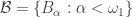 be a base for
  , which is a base for
  . Since
  . Furthermore,
  .
. . We can assume that
  . Let
. Let  for some
  . Since
  for some finite
  . Note that
  and that
  .
. . Since
  . Furthermore, for any countable
  ,
, ![[(\bigcap_{\beta<\alpha} U_\beta) \cap (\bigcap_{n \in \omega} X^2 \backslash \{ y_n \}) ]\backslash \Delta \ne \varnothing](https://s0.wp.com/latex.php?latex=%5B%28%5Cbigcap_%7B%5Cbeta%3C%5Calpha%7D+U_%5Cbeta%29+%5Ccap+%28%5Cbigcap_%7Bn+%5Cin+%5Comega%7D+X%5E2+%5Cbackslash+%5C%7B+y_n+%5C%7D%29+%5D%5Cbackslash+%5CDelta+%5Cne+%5Cvarnothing&bg=ffffff&fg=333333&s=0&c=20201002) .
. . For any
  , choose
  .
. converges to the diagonal
  . From the way the sequence is chosen,
  for all
  . This concludes the proof that
  . Then if
  and thus
  , i.e.
  is a free sequence of length
  if for each
  ,
,  . For any compact space with tightness at least
  .
. contains all but countably many
  . Consider the sequence
 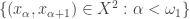 . Observe that every open set in
  contains all but countably pairs
  . This implies that every open set containing the diagonal
 ![\omega_1+1=[0, \omega_1]](https://s0.wp.com/latex.php?latex=%5Comega_1%2B1%3D%5B0%2C+%5Comega_1%5D&bg=ffffff&fg=333333&s=0&c=20201002) does not have a small diagonal since it is uncountably tight at the last point
does not have a small diagonal since it is uncountably tight at the last point ![D=[0,1] \times \{0, 1 \}](https://s0.wp.com/latex.php?latex=D%3D%5B0%2C1%5D+%5Ctimes+%5C%7B0%2C+1+%5C%7D&bg=ffffff&fg=333333&s=0&c=20201002) . The space
. The space  consists of two copies of the unit interval, an upper one and a lower one. See the first two diagrams in
  , a basic open set containing the point
  in the upper interval is of the form
 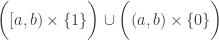 . For
. For  , a basic open set containing the point
  in the lower interval is of the form
 ![\biggl( (c,a) \times \{ 1 \} \biggr) \cup \biggl( (c,a] \times \{0 \} \biggr)](https://s0.wp.com/latex.php?latex=%5Cbiggl%28+%28c%2Ca%29+%5Ctimes+%5C%7B+1+%5C%7D+%5Cbiggr%29+%5Ccup+%5Cbiggl%28+%28c%2Ca%5D+%5Ctimes+%5C%7B0+%5C%7D+%5Cbiggr%29&bg=ffffff&fg=333333&s=0&c=20201002) . The rightmost point in the upper interval
. The rightmost point in the upper interval  and the leftmost point in the lower interval
  are made isolated points.
 such that each point inverse is metrizable.
 ![f:D \rightarrow [0,1]](https://s0.wp.com/latex.php?latex=f%3AD+%5Crightarrow+%5B0%2C1%5D&bg=ffffff&fg=333333&s=0&c=20201002) be defined by
be defined by  for each
  . This is a two-to-one continuous map from the double arrow space
  as one point
  such that
  -weight.
![I=[0,1]](https://s0.wp.com/latex.php?latex=I%3D%5B0%2C1%5D&bg=ffffff&fg=333333&s=0&c=20201002) be the closed unit interval with the usual topology. Let
be the closed unit interval with the usual topology. Let  be the set of all functions
  . The set
  or
or  where each
  . As a product of compact spaces,
  is compact.
  for all
  (such a function is usually referred to as non-decreasing). Helly space is the subspace
  is normal.
 is Example 106 in [2]. This product is not normal. The non-normality of
  is normal if and only if the compact space
  defined as follows:
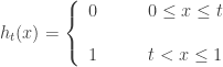
 . Let
. Let  . Consider the mapping
  defined by
  . With the domain
  having the Sorgenfrey topology and with the range
  being a subspace of Helly space, it can be shown that
  is a homeomorphism.
 contains a copy of the Sorgenfrey plane
  , which is non-normal (discussed

 is a closed subset of
  , define
  as follows:
 . The set
  ,
,  (closure taken in
  be a countable base for the usual topology on the unit interval


 and for each
  with
with  , we would like to arrange the elements in increasing order, notated as follow:
 . For the set
  ,
,  is to the left of
  for
for  . Note that elements of
  . If
. If  , then
  . If
. If  , then
 ![E_n=(p_n,q_n]=(p_n,1]](https://s0.wp.com/latex.php?latex=E_n%3D%28p_n%2Cq_n%5D%3D%28p_n%2C1%5D&bg=ffffff&fg=333333&s=0&c=20201002) .
. as follows:
 when both
 is not hereditarily normal (see Theorem 3 in
  or
or  . In fact, for any compact non-metric space
 be a space. It is submetrizable if there is a topology
  on the set
  and
and  is a metrizable space. The topology
  be a set of subsets of the space
  such that
  . Having a network that is countable in size is a strong property (see
  of the square
  is clear. For
  , see Lemma 1 in
  is left as an exercise. To see
  , let
, let  . This follows from the well known result that any countably compact space with a
  (see
(see  and
and  .
.![[0,\alpha]](https://s0.wp.com/latex.php?latex=%5B0%2C%5Calpha%5D&bg=ffffff&fg=333333&s=0&c=20201002) which is metrizable. Any Moore space has a
which is metrizable. Any Moore space has a  is the space of all continuous functions from
  is metrizable and separable since it is a subspace of the separable metric space
  . Thus
  be a countable base for
  be the restriction map, i.e. for each
  ,
,  . Since
  .
.  , and for
  , there exists
  such that
  . Since
  function space theory. More about this point later. First, consider a corollary of Theorem 1.
 where
where  is the cardinality continuum and each
  is a product of separable spaces where
  , is the least cardinaility of a base of
  , there is an open subset
  and
and  is compact. When we say
  where each
  is a locally compact space. In proving the result discussed here, we also assume that each
  of
of  is a locally finite family consisting of compact sets.
 such that each
  is closed and is locally compact. Fix an integer
  , let
, let  be an open subset of
  and
and  is compact (the closure is taken in
  of
of  be a locally finite open cover of
  for each
  is compact since
  . Let
. Let  .
. is a locally finite family with respect to the space
  ,
,  is an open set containing
  that meets only finitely many sets in
  . It is clear that
  be a
be a  and for each
  is obviously compact.
  , the point
  for some
  . Choose open
  and open
  such that
  . Letting
  cover the compact set
  be the intersection of these finitely many
  . Let
. Let  be the set of these finitely many
  .
. ,
, ,
,  for some
  such that
  for all

 . Then for some
  for some
  . Furthermore,
  for some
  . We now have
  .
. . Immediately we see that
  .
. is a locally finite family of open subsets of
  such that
  and
and  meets only finitely many sets in
  . Recall that
  is the set of all
  and is locally finite. Thus there exists an open
  and
and  . Thus the open set
  for finitely many
  meets only finitely many sets
  in
in 
 be the Michael line. Let
  be the space of the irrational numbers. The space
 is a continuous function, then
  is a bounded set in the real line. Compact spaces are pseudocompact. In fact, it is clear from definitions that
 where
where  is a maximal almost disjoint family of subsets of
  be a one-to-one continuous function from
  . Then
  is a homeomorphism.
 are countably many compact spaces such that each
  has at least two points. If each
  is countably tight.
 ,
,  , and
, and  , then
  .
. be a continuous and closed map from the space
  onto the space
  . Suppose that the space
  and
and  where
where  . We proceed to find a countable
  such that
  . Choose
  such that
  . By assumption,
  countably reached by
  such that
  . Let
. Let  . Let
. Let  be open such that
  . Because the space
  such that
  and
and  . Then
  . Furthermore,
  . Let
. Let  . According to the fact about continuity stated above, we have
  . Since
  such that
  . Choose a countable
  such that
  . It follows that
  .
. . Since
  , we have
  . Note that
  is a closed set since
  . As a result,
  . Then
  for some
  . We have
  .
. . With
  . Thus,
  . Note that the arbitrary open neighborhood
  ,
,  and
and  such that
  . For each
  , choose a countable
  with
with  . Let
. Let  . Note that
  and
and  be the projection map. If
  . It follows that no point of
  belongs to
  of
of  and
and  . The set of all
  for
for  .
. . We have
  . Since
  such that
  . It follows that
  . Choose
  . Then for some
  . Since
  ,
,  , implying that
  , a contradiction. Thus
  be the projection map. The projection map is always continuous. Furthermore it is a closed map by Lemma 5. The range space
  is a closed subspace of a
  where
where  . The
. The  with
with 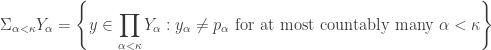
 depends on the base point
  .
. for all
  to denote the
  contains
  , let
, let  , where for each
  and that
  if
if  . For each
  , let
, let  . By Theorem 7, each
  is normal. Let
  , which is also normal. By Theorem 6, the space
  . Let
. Let  . We have the following derivation.
 is defined such that for each
  and for each
  ,
,  . Furthermore, for
  , for each
  , let
, let  . Thus
 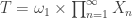 is a closed subspace of the normal space
  must be countably tight.
  .
.
 is a point of
  for all
  . When the countable product space is countably tight, the finite product, being a subspace of a countably tight space, is also countably tight.
 for all
  ,
, for all
 for all


 is the product of
  where
where  cannot be hereditarily normal as long as there are uncountably many factors and every factor has at least two point.
 are hereditarily normal can tell us whether
  is not metrizable since it is not first countable (see Problem 1 below). Thus one of its first three self products must fail to be hereditarily normal.
  be a set with cardinality
  . Show that
  .
. is a
is a  and that it has only finitely many coordinates at which
  .
. be the set of non-negative integers with the discrete topology. Show that the product space
  . Show that

 has a countably infinite subspace that is relatively discrete (see Problem 6). In other words, it has a subspace that is homemorphic to
  where
where 
 is hereditarily normal (i.e. every one of its subspaces is normal), then one of the following condition holds:
 is perfectly normal.
 is closed.
 were to be hereditarily normal, then the first condition must be satisfied, i.e.
  is hereditarily normal, then
 .
.