Perfect images of separable metric spaces

Posted on March 28, 2023 by Dan Ma

The Bow-Tie space is the continuous image of a separable metric space and yet is not metrizable (see here). Though taking continuous image can fail to preserve separable metrizability, we show that the perfect image of a separable metric space is a separable metric space. We prove the following theorem, which says that under a perfect map the weight will not increase. The result about separable metric space is a corollary of Theorem 1.

Theorem 1
Let $f:X \longrightarrow Y$ be a perfect map onto the space $Y$ . Then $w(Y) \le w(X)$ , i.e., the weight of $Y$ is no greater than the weight of $X$ .

Proof of Theorem 1

All spaces under consideration are Hausdorff. Let $X$ and $Y$ be spaces. Let $f: \longrightarrow Y$ be a map (or function) from $X$ onto $Y$ . The map $f$ is said to be a closed map if $f(C)$ is closed in $Y$ for any closed subset $C$ of $X$ . The map $f$ is a perfect map if $f$ is continuous, $f$ is a closed map, and $f^{-1}(y)$ is compact for every $y \in Y$ . In words, the last condition is that every point inverse is compact. A point inverse $f^{-1}(y)$ is also referred to as a fiber. Thus, we can say that a perfect map is a continuous closed surjective map with compact fibers. The following lemma is helpful for proving Theorem 1.

Lemma 2
Let $f:X \longrightarrow Y$ be a closed map such that $f(X)=Y$ . Let $V \subset X$ be open. Let $f_*(V)=\{ y \in Y: f^{-1}(y) \subset V \}$ . Then $f_*(V)$ is open in $Y$ and $f_*(V) \subset f(V)$ .

Proof of Lemma 2
We show that $Y \backslash f_*(V)$ is closed in $Y$ . To this end, we show $f(X \backslash V)=Y \backslash f_*(V)$ . Note that $f(X \backslash V)$ is closed in $Y$ since $f$ is a closed map. First, we show $f(X \backslash V) \subset Y \backslash f_*(V)$ . Let $t \in f(X \backslash V)$ . Then $t=f(x)$ for some $x \in X \backslash V$ . Since $x \notin V$ and $x \in f^{-1}(t)$ , we have $f^{-1}(t) \not \subset V$ . This implies that $t \notin f_*(V)$ .

We now show that $Y \backslash f_*(V) \subset f(X \backslash V)$ . Let $z \in Y \backslash f_*(V)$ . Since $z \notin f_*(V)$ , $f^{-1}(z) \not \subset V$ . Choose $x \in f^{-1}(z) \backslash V$ , which implies that $x \in X \backslash V$ . Thus, $z=f(x) \in f(X \backslash V)$ .

To complete the proof of the lemma, we show $f_*(V) \subset f(V)$ . Let $w \in f_*(V)$ . We have $f^{-1}(w) \subset V$ . As a result, $w=f(x)$ for some $x \in V$ . $\square$

Proof of Theorem 1
Let $\mathcal{B}$ be a base for $X$ . We derive a base $\mathcal{B}_1$ for $Y$ such that $\lvert \mathcal{B}_1 \lvert \le \lvert \mathcal{B} \lvert$ , i.e., the cardinality of $\mathcal{B}_1$ is no more than the cardinality of $\mathcal{B}$ . This implies that the minimal cardinality of a base in $Y$ is no more than the minimal cardinality of a base in $X$ , i.e., $w(Y) \le w(X)$ .

We assume that the base $\mathcal{B}$ is closed under finite unions. We show that $\mathcal{B}_1=\{ f_*(B): B \in \mathcal{B} \}$ is a base for $Y$ . Note that $f_*$ is defined in Lemma 2. Let $U \subset Y$ be an open set. Let $y \in U$ . For each $x \in f^{-1}(y)$ , choose $B_x \in \mathcal{B}$ such that $x \in B_x$ and $f(B_x) \subset U$ . Since $f^{-1}(y)$ is compact, there exists finite $F \subset f^{-1}(y)$ such that $f^{-1}(y) \subset \bigcup_{t \in F} B_t=B$ . Note that $B \in \mathcal{B}$ . Since $f^{-1}(y) \subset B$ , we have $y \in f_*(B)$ . We also have $f_*(B) \subset f(B) \subset U$ . Thus, every open subset $U$ of $Y$ is the union of elements of $\mathcal{B}_1$ . This means that $\mathcal{B}_1$ is a base for $Y$ . Theorem 1 is established. $\square$

Corollary 3
Let $f:X \longrightarrow Y$ be a perfect map onto the space $Y$ . Then if $X$ is a separable metric space, then $Y$ is a separable metric space.

Comment About Lemma 2
A perfect map is not necessarily an open map. If the perfect map $f$ in Theorem 1 is an open map, then Lemma 2 is not needed and $\mathcal{B}_1=\{ f(B): B \in \mathcal{B} \}$ would be a base for $Y$ . However, we cannot assume $f$ is an open map simply because it is a perfect map. To see this, let $X=\mathbb{R}$ be the real line with the usual topology. Collapse the closed interval $[1,2]$ to one point called $p$ . The resulting quotient space is $Y$ where $Y=(-\infty,1) \cup \{ p \} \cup (2,\infty)$ . In $Y$ , the open neighborhoods of points in $(-\infty,1) \cup (2,\infty)$ are the usual Euclidean neighborhoods. The open neighborhoods of the point $p$ are the usual Euclidean open sets containing the interval $[1,2]$ . The resulting quotient map $f$ is an identity map on $(-\infty,1) \cup (2,\infty)$ and it maps points in $[1,2]$ to the point $p$ . It can be verified that $f$ is a perfect map. For the open set $V=(1,2)$ , $f(V)=\{ p \}$ , which is not open in $Y$ . For the open set $V=(0,1.5)$ , $f(V)=(0,1) \cup \{ p \}$ , which is not open in $Y$ . Lemma 2 says that for any open $X \subset$ , $f(V)$ may not be open but has an open subset $f_*(V)$ if $f(V)$ has non-empty interior. The interior sets $f_*(V)$ can work as a base in $Y$ .

Invariant and Inverse Invariant

Let $\mathcal{P}$ be a property of topological spaces. We say that $\mathcal{P}$ is an invariant of the perfect maps or that $\mathcal{P}$ is invariant under the perfect maps if the property $\mathcal{P}$ is preserved by perfect maps, i.e., for each perfect map $f:X \longrightarrow Y$ where $Y=f(X)$ , if the space $X$ has $\mathcal{P}$ , so does $Y$ . On the other hand, $\mathcal{P}$ is an inverse invariant of the perfect maps if this holds: for each perfect map $f:X \longrightarrow Y$ where $Y=f(X)$ , if $Y$ has $\mathcal{P}$ , so does $X$ .

The notions invariant and inverse invariant defined here are for perfect maps. In general, the notions are much broader and can be defined in relation to any class of continuous maps. For example, we know that the continuous image of a separable space is separable. We can say that separability is an invariant of the continuous maps or that separability is invariant under continuous maps. We can now restate Theorem 1 and Corollary 3 as follows.

Theorem 4…..Restatement of Theorem 1
The property “weight $\le \mathcal{K}$ ” is an invariant of the perfect maps.

Corollary 5
The second axiom of countability is invariant under the perfect maps, but is not an invariant of the continuous maps.

The Bow-Tie space is the continuous image of a separable space but cannot have a countable base (see here). In light of Theorem 1, the continuous map that maps a separable metric space to the Bow-Tie space (shown here) cannot be a perfect map. With respect to that map, the upper half plane in the domain (the separable metric space) is closed but its continuous image in the Bow-Tie space is open and not closed.

$\text{ }$

Dan Ma Bow-Tie space
Daniel Ma Bow-Tie space

Dan Ma perfect map
Daniel Ma perfect map

Dan Ma separable metric space
Daniel Ma separable metric space

Dan Ma topology
Daniel Ma topology

$\copyright$ 2023 – Dan Ma

Revised March 31, 2023
Revised March 12, 2024

The Bow-Tie Space

Posted on March 26, 2023 by Dan Ma

We present the Bow-Tie space, which exhibits many interesting properties. The Bow-Tie space is hereditarily Lindelof, and hereditarily separable. It is also the continuous image of a separable metric space. These properties follow from the fact that the Bow-Tie space has a countable network. Furthermore, the Bow-Tie space is neither metrizable nor a Moore space. Thus, the example demonstrates that the continuous image of a separable metric space does not have to be a separable metric space.

Louis F. McAuley introduced the Bow-Tie space as an example of a regular semimetric space that is hereditarily separable, collectionwise normal, completely normal and paracompact, but is not second countable and is not developable, hence not a Moore space [3]. The Bow-Tie space is also discussed in Counterexamples in Topology [5] (see p. 175 Dover Edition). In these two references, the Bow-Tie space is defined as a semimetric space. The version given here is found in [4]. The Bow-Tie space is given in [4] as an example of a cosmic space (i.e., a space with a countable network) that is not an $\aleph_0$ -space.

All spaces under consideration are Hausdorff. Let $X$ be a space. A collection $\mathcal{N}$ of subsets of $X$ is said to be a network for $X$ if for each $x \in X$ and for each open set $O$ containing $x$ , there exists $A \in \mathcal{N}$ such that $x \in A \subset O$ . A network behaves like a base but the elements of the network do not have to be open sets. Of interest are the spaces with a countable network. Compact spaces with a countable network is metrizable. Any space with a countable network is both hereditarily separable and hereditarily Lindelof. The space $X$ has a countable network if and only if $X$ is the continuous image of a separable metric space. Having a countable network is a strong property. See here for a discussion of these facts about spaces with countable network.

The Bow-Tie Space

Let $Y$ be the upper half plane, which is the set of all pairs of real numbers $(x,y)$ with $y>0$ . Let $H$ be the x-axis, which is the set of all pairs of real numbers $(x,y)$ with $y=0$ . The bow-tie space is the set $X=Y \cup H$ with the topology defined as follows.

Open neighborhoods of points in the upper half plane $Y$ are the Euclidean open subsets of $Y$ .
An open neighborhood of a point $p$ in the x-axis $H$ is of the form $B(p,c)$ with $0<c \le 1$ . Each set $B(p,c)$ consists of the point $p$ and all points $q \in X$ having Euclidean distance less than $c$ from $p$ and lying underneath either one of the two straight lines emanating from $p$ with slopes $c$ and $-c$ , respectively.

In the following diagram, $B(p,c)$ is represented by the area in the upper half plane shaded in green plus the points in the x-axis having a distance less than $c$ from $p$ and below the two lines with slopes $c$ and $-c$ .

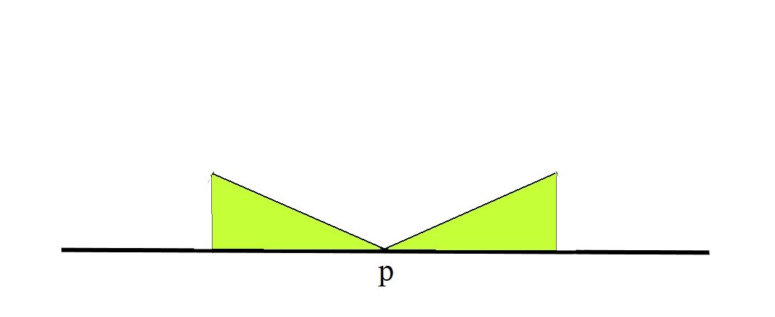
It is straightforward to verify that the open neighborhoods produce a Hausdorff and regular space. The relative Bow-Tie topologies on $Y$ and $H$ coincide with the Euclidean topologies on $Y$ and $H$ , respectively. Let $\mathcal{B}_1$ and $\mathcal{B}_2$ be countable bases for $Y$ and $H$ in their respective relative Euclidean topologies. Then $\mathcal{N}=\mathcal{B}_1 \cup \mathcal{B}_2$ is a network for the Bow-Tie space $X$ . Thus, the Bow-Tie space has a countable network. Any space with a countable network is Lindelof and separable. The property of having a countable netowrk is hereditary. Thus, the Bow-Tie space is hereditarily Lindelof and hereditarily separable. See here for a discussion of these facts about spaces with countable network.

Any space with a countable network is the continuous image of a separable metric space. In the case of the Bow-Tie space, we can see this directly. Let $Y_1$ be the upper half plane $Y$ with the Euclidean topology. Let $H_1$ be the x-axis $H$ with the Euclidean topology. Let $X_1=Y_1 \bigoplus H_1$ , the free sum or free union. This means that $U \subset X_1$ is open if and only if both $U \cap Y_1$ and $U \cap H_1$ are open. It follows that the identity map from $X_1$ onto the Bow-Tie space $X$ is continuous.

The Bow-Tie space $X$ is separable but not metrizable. We show that $X$ does not have a countable base. Suppose it does. Let $\mathcal{B}$ be a countable base for the Bow-Tie space. We can assume that the elements of $\mathcal{B}$ that contain points of the x-axis $H$ are of the form $B(p,c)$ defined above. Since $\mathcal{B}$ is countable, there can only be countably many $B(p,c)$ in $\mathcal{B}$ , say, $B(p_0,c_0)$ , $B(p_1,c_1)$ , $B(p_2,c_2)$ , $B(p_3,c_3),\cdots$ . Pick $p \in H$ such that $p \ne p_i$ for all $i$ . Consider $B(p,1)$ . Since $\mathcal{B}$ is a base, there must exist some $i$ such that $p \in B(p_i,c_i) \subset B(p,1)$ . This means that both the left side and the right side of the bow-tie in $B(p_i,c_i)$ are within $B(p,1)$ . On the other hand, one side of the bow-tie of $B(p_i,c_i)$ (either the left side or the right side) is above the point $p$ . The points on that side of the bow-tie of $B(p_i,c_i)$ right above point $p$ cannot be part of $B(p,1)$ , a contradiction. Thus, the Bow-Tie space $X$ cannot have a countable base and hence not metrizable. The Bow-Tie space cannot be a Moore space since any Lindelof Moore space must have a countable base.

Not only the Bow-Tie space cannot have a countable base, it also cannot have a point-countable base. For any space, a base is a point-countable base if every point in the space belongs to only countably many elements of the base. In [3] and [5], the Bow-Tie space is defined using a semimetric. Heath [2] showed that every semimetric space with a point-countable base is developable, hence a Moore space if the space is regular. The Bow-Tie space cannot have a point-countable base. If it does, it would be a Moore space.

We mention two more facts about the Bow-Tie space. One is that the Bow-Tie space is a Lindelof $\Sigma$ -space. It is well known that any space with a countable network is a Lindelof $\Sigma$ -space [6]. Secondly, $C_p(X)$ , the function space with the pointwise convergence topology on the Bow-Tie space $X$ is a hereditarily D-space. Gruenhage [1] showed that if $L$ is a Lindelof $\Sigma$ -space, then $C_p(L)$ is a hereditarily D-space.

Reference

Gruenhage, G., A note on D-spaces, Topology and Appl. 152, 2229-2240, 2006.
Heath, R. W., On spaces with point-countable bases, Bull. Acad. Polon. Sci. 13, 393-395, 1965.
McAuley, L. F., A relation between perfect separability, completeness, and normality in semimetric spaces, Pacific J. Math. 6, 315-326, 1956.
Michael, E., $\aleph_0$ -spaces, J. Math. Mech., 15, 983-1002, 1966.
Steen, L. A., Seebach, J. A., Counterexamples in Topology, Dover Publications, Inc., New York, 1995.
Tkachuk, V. V., Lindelof $\Sigma$ -spaces: an omnipresent class, RACSAM, 104 (2), 221-244, 2010.

$\text{ }$

Dan Ma Bow-Tie space
Daniel Ma Bow-Tie space

Dan Ma hereditarily Lindelof space
Daniel Ma hereditarily Lindelof space

Dan Ma hereditarily separable space
Daniel Ma hereditarily separable space

Dan Ma countable network
Daniel Ma countable network

Dan Ma topology
Daniel Ma topology

$\copyright$ 2023 – Dan Ma

Sigma-products of separable metric spaces are monolithic

Posted on June 3, 2014 by Dan Ma

Let $\Sigma(\kappa)$ be the $\Sigma$ -product of $\kappa$ many copies of the real lines where $\kappa$ is any infinite cardinal number. Any compact space that can be embedded in $\Sigma(\kappa)$ for some $\kappa$ is said to be a Corson compact space. Corson compact spaces play an important role in functional analysis. Corson compact spaces are also very interesting from a topological point of view. Some of the properties of Corson compact spaces are inherited (as subspaces) from the $\Sigma$ -product $\Sigma(\kappa)$ . One such property is the property that the $\Sigma$ -product $\Sigma(\kappa)$ is monolithic, which implies that the closure of any countable subspace of $\Sigma(\kappa)$ is metrizable.

Previous blog posts on $\Sigma$ -products:

A previous blog post on monolithic spaces: A short note on monolithic spaces. A listing of other blog posts on Corson compact spaces is given at the end of this post.

____________________________________________________________________

Defining Sigma-product

Let $\kappa$ be an infinite cardinal number. For each $\alpha<\kappa$ , let $X_\alpha$ be a topological space. Let $b \in \prod_{\alpha<\kappa} X_\alpha$ . The $\Sigma$ -product of the spaces $X_\alpha$ about the base point $b$ is defined as follows:

$\Sigma_{\alpha<\kappa} X_\alpha=\left\{x \in \prod_{\alpha<\kappa} X_\alpha: x_\alpha \ne b_\alpha \text{ for at most countably many } \alpha < \kappa \right\}$

If each $X_\alpha=\mathbb{R}$ and if the base point $b$ is such that $b_\alpha=0$ for all $\alpha<\kappa$ , then we use the notation $\Sigma(\kappa)$ for $\Sigma_{\alpha<\kappa} X_\alpha$ , i.e., $\Sigma(\kappa)$ is defined as follows:

$\Sigma(\kappa)=\left\{x \in \mathbb{R}^\kappa: x_\alpha \ne 0 \text{ for at most countably many } \alpha < \kappa \right\}$

A compact space is said to be a Corson compact space if it can be embedded in the $\Sigma$ -product $\Sigma(\kappa)$ for some infinite cardinal $\kappa$ .

____________________________________________________________________

Monolithic Spaces

A space $X$ is monolithic if for every subspace $Y$ of $X$ , the density of $Y$ equals the network weight of $Y$ , i.e., $d(Y)=nw(Y)$ . A space $X$ is strongly monolithic if for every subspace $Y$ of $X$ , the density of $Y$ equals the weight of $Y$ , i.e., $d(Y)=w(Y)$ . See the previous post called A short note on monolithic spaces.

The proof of the fact that $\Sigma$ -product of separable metrizable spaces is monolithic can be worked out quite easily from definitions. Interested readers are invited to walk through the proof. For the sake of completeness, we prove the following theorem.

Theorem 1
Suppose that for each $\alpha<\kappa$ , $X_\alpha$ is a separable metric space. Then the $\Sigma$ -product $\Sigma_{\alpha<\kappa} X_\alpha$ is strongly monolithic.

Proof of Theorem 1
Let $b$ be the base point of the $\Sigma$ -product $X=\Sigma_{\alpha<\kappa} X_\alpha$ . For each $x \in X$ , let $S(x)$ be the support of the point $x$ , i.e., the set of all $\alpha<\kappa$ such that $x_\alpha \ne b_\alpha$ . Let Y be a subspace of $X$ . We show that $d(Y)=w(Y)$ .

Let $T=\left\{t_\delta: \delta<\tau \right\}$ be a dense subspace of $Y$ such that $d(Y)=\lvert T \lvert=\tau$ . Note that $\overline{T}=Y$ (closure is taken in $Y$ ). Let $S=\bigcup_{\delta<\tau} S(t_\delta)$ . Clearly $\lvert S \lvert \le \tau$ . Consider the following subspace of $X$ :

$X(S)=\left\{x \in X: S(x) \subset S \right\}$

It is clear that $X(S)$ is a closed subspace of $X$ . Since $T \subset X(S)$ , the closure of $T$ (closure in $X$ or in $Y$ ) is a subspace of $X(S)$ . Thus $Y \subset X(S)$ . Note that $\overline{T}=Y \subset X(S)$ . Since each $X_\alpha$ has a countable base, the product space $\prod_{\alpha<\tau} X_\alpha$ has a base of cardinality $\tau$ . Thus $\prod_{\alpha<\tau} X_\alpha$ has weight $\le \tau$ . Since $X(S) \subset \prod_{\alpha<\tau} X_\alpha$ , both $Y$ and $X(S)$ have weights $\le \tau$ . We have $w(Y) \le d(Y)=\tau$ . Note that $d(Y) \le w(Y)$ always holds. Therefore $d(Y)=w(Y)$ . $\blacksquare$

Corollary 2
For any infinite cardinal $\kappa$ , the $\Sigma$ -product $\Sigma(\kappa)$ is strongly monolithic.

Corollary 3
Any Corson compact space is strongly monolithic.

____________________________________________________________________

Blog posts on Corson compact spaces

____________________________________________________________________
$\copyright \ 2014 \text{ by Dan Ma}$

(Lower case) sigma-products of separable metric spaces are Lindelof

Posted on April 21, 2014 by Dan Ma

Consider the product space $X=\prod_{\alpha \in A} X_\alpha$ . Fix a point $b \in \prod_{\alpha \in A} X_\alpha$ , called the base point. The $\Sigma$ -product of the spaces $\left\{X_\alpha: \alpha \in A \right\}$ is the following subspace of the product space $X$ :

$\Sigma_{\alpha \in A} X_\alpha=\left\{ x \in X: x_\alpha \ne b_\alpha \text{ for at most countably many } \alpha \in A \right\}$

In other words, the space $\Sigma_{\alpha \in A} X_\alpha$ is the subspace of the product space $X=\prod_{\alpha \in A} X_\alpha$ consisting of all points that deviate from the base point on at most countably many coordinates $\alpha \in A$ . We also consider the following subspace of $\Sigma_{\alpha \in A} X_\alpha$ .

$\sigma=\left\{ x \in \Sigma_{\alpha \in A} X_\alpha: x_\alpha \ne b_\alpha \text{ for at most finitely many } \alpha \in A \right\}$

For convenience , we call $\Sigma_{\alpha \in A} X_\alpha$ the (upper case) Sigma-product (or $\Sigma$ -product) of the spaces $X_\alpha$ and we call the space $\sigma$ the (lower case) sigma-product (or $\sigma$ -product). Clearly, the space $\sigma$ is a dense subspace of $\Sigma_{\alpha \in A} X_\alpha$ . In a previous post, we show that the upper case Sigma-product of separable metric spaces is collectionwise normal. In this post, we show that the (lower case) sigma-product of separable metric spaces is Lindelof. Thus when each factor $X_\alpha$ is a separable metric space with at least two points, the $\Sigma$ -product, though not Lindelof, has a dense Lindelof subspace. The (upper case) $\Sigma$ -product of separable metric spaces is a handy example of a non-Lindelof space that contains a dense Lindelof subspace.

Naturally, the lower case sigma-product can be further broken down into countably many subspaces. For each integer $n=0,1,2,3,\cdots$ , we define $\sigma_n$ as follows:

$\sigma_n=\left\{ x \in \sigma: x_\alpha \ne b_\alpha \text{ for at most } n \text{ many } \alpha \in A \right\}$

Clearly, $\sigma=\bigcup_{n=0}^\infty \sigma_n$ . We prove the following theorem. The fact that $\sigma$ is Lindelof will follow as a corollary. Understanding the following proof for Theorem 1 is a matter of keeping straight the notations involving standard basic open sets in the product space $X=\prod_{\alpha \in A} X_\alpha$ . We say $V$ is a standard basic open subset of the product space $X$ if $V$ is of the form $V=\prod_{\alpha \in A} V_\alpha$ such that each $V_\alpha$ is an open subset of the factor space $X_\alpha$ and $V_\alpha=X_\alpha$ for all but finitely many $\alpha \in A$ . The finite set $F$ of all $\alpha \in A$ such that $V_\alpha \ne X_\alpha$ is called the support of the open set $V$ .

Theorem 1
Let $\sigma$ be the $\sigma$ -product of the separable metrizable spaces $\left\{X_\alpha: \alpha \in A \right\}$ . For each $n$ , let $\sigma_n$ be defined as above. The product space $\sigma_n \times Y$ is Lindelof for each non-negative integer $n$ and for all separable metric space $Y$ .

Proof of Theorem 1
We prove by induction on $n$ . Note that $\sigma_0=\left\{b \right\}$ , the base point. Clearly $\sigma_0 \times Y$ is Lindelof for all separable metric space $Y$ . Suppose the theorem hold for the integer $n$ . We show that $\sigma_{n+1} \times Y$ for all separable metric space $Y$ . To this end, let $\mathcal{U}$ be an open cover of $\sigma_{n+1} \times Y$ where $Y$ is a separable metric space. Without loss of generality, we assume that each element of $\mathcal{U}$ is of the form $V \times W$ where $V=\prod_{\alpha \in A} V_\alpha$ is a standard basic open subset of the product space $X=\prod_{\alpha \in A} X_\alpha$ and $W$ is an open subset of $Y$ .

Let $\mathcal{U}_0=\left\{U_1,U_2,U_3,\cdots \right\}$ be a countable subcollection of $\mathcal{U}$ such that $\mathcal{U}_0$ covers $\left\{b \right\} \times Y$ . For each $j$ , let $U_j=V_j \times W_j$ where $V_j=\prod_{\alpha \in A} V_{j,\alpha}$ is a standard basic open subset of the product space $X$ with $b \in V_j$ and $W_j$ is an open subset of $Y$ . For each $j$ , let $F_j$ be the support of $V_j$ . Note that $\alpha \in F_j$ if and only if $V_{j,\alpha} \ne X_\alpha$ . Also for each $\alpha \in F_j$ , $b_\alpha \in V_{j,\alpha}$ . Furthermore, for each $\alpha \in F_j$ , let $V^c_{j,\alpha}=X_\alpha- V_{j,\alpha}$ . With all these notations in mind, we define the following open set for each $\beta \in F_j$ :

$H_{j,\beta}= \biggl( V^c_{j,\beta} \times \prod_{\alpha \in A, \alpha \ne \beta} X_\alpha \biggr) \times W_j=\biggl( V^c_{j,\beta} \times T_\beta \biggr) \times W_j$

Observe that for each point $y \in \sigma_{n+1}$ such that $y \in V^c_{j,\beta} \times T_\beta$ , the point $y$ already deviates from the base point $b$ on one coordinate, namely $\beta$ . Thus on the coordinates other than $\beta$ , the point $y$ can only deviates from $b$ on at most $n$ many coordinates. Thus $\sigma_{n+1} \cap (V^c_{j,\beta} \times T_\beta)$ is homeomorphic to $V^c_{j,\beta} \times \sigma_n$ . Note that $V^c_{j,\beta} \times W_j$ is a separable metric space. By inductive hypothesis, $V^c_{j,\beta} \times \sigma_n \times W_j$ is Lindelof. Thus there are countably many open sets in the open cover $\mathcal{U}$ that covers points of $H_{j,\beta} \cap (\sigma_{n+1} \times W_j)$ .

Note that

$\sigma_{n+1} \times Y=\biggl( \bigcup_{j=1}^\infty U_j \cap \sigma_{n+1} \biggr) \cup \biggl( \bigcup \left\{H_{j,\beta} \cap (\sigma_{n+1} \times W_j): j=1,2,3,\cdots, \beta \in F_j \right\} \biggr)$

To see that the left-side is a subset of the right-side, let $t=(x,y) \in \sigma_{n+1} \times Y$ . If $t \in U_j$ for some $j$ , we are done. Suppose $t \notin U_j$ for all $j$ . Observe that $y \in W_j$ for some $j$ . Since $t=(x,y) \notin U_j$ , $x_\beta \notin V_{j,\beta}$ for some $\beta \in F_j$ . Then $t=(x,y) \in H_{j,\beta}$ . It is now clear that $t=(x,y) \in H_{j,\beta} \cap (\sigma_{n+1} \times W_j)$ . Thus the above set equality is established. Thus one part of $\sigma_{n+1} \times Y$ is covered by countably many open sets in $\mathcal{U}$ while the other part is the union of countably many Lindelof subspaces. It follows that a countable subcollection of $\mathcal{U}$ covers $\sigma_{n+1} \times Y$ . $\blacksquare$

Corollary 2
It follows from Theorem 1 that

If each factor space $X_\alpha$ is a separable metric space, then each $\sigma_n$ is a Lindelof space and that $\sigma=\bigcup_{n=0}^\infty \sigma_n$ is a Lindelof space.
If each factor space $X_\alpha$ is a compact separable metric space, then each $\sigma_n$ is a compact space and that $\sigma=\bigcup_{n=0}^\infty \sigma_n$ is a $\sigma$ -compact space.

Proof of Corollary 2
The first bullet point is a clear corollary of Theorem 1. A previous post shows that $\Sigma$ -product of compact spaces is countably compact. Thus $\Sigma_{\alpha \in A} X_\alpha$ is a countably compact space if each $X_\alpha$ is compact. Note that each $\sigma_n$ is a closed subset of $\Sigma_{\alpha \in A} X_\alpha$ and is thus countably compact. Being a Lindelof space, each $\sigma_n$ is compact. It follows that $\sigma=\bigcup_{n=0}^\infty \sigma_n$ is a $\sigma$ -compact space. $\blacksquare$

____________________________________________________________________

A non-Lindelof space with a dense Lindelof subspace

Now we put everything together to obtain the example described at the beginning. For each $\alpha \in A$ , let $X_\alpha$ be a separable metric space with at least two points. Then the $\Sigma$ -product $\Sigma_{\alpha \in A} X_\alpha$ is collectionwise normal (see this previous post). According to the lemma in this previous post, the $\Sigma$ -product $\Sigma_{\alpha \in A} X_\alpha$ contains a closed copy of $\omega_1$ . Thus the $\Sigma$ -product $\Sigma_{\alpha \in A} X_\alpha$ is not Lindelof. It is clear that the $\sigma$ -product is a dense subspace of $\Sigma_{\alpha \in A} X_\alpha$ . By Corollary 2, the $\sigma$ -product is a Lindelof subspace of $\Sigma_{\alpha \in A} X_\alpha$ .

Using specific factor spaces, if each $X_\alpha=\mathbb{R}$ with the usual topology, then $\Sigma_{\alpha<\omega_1} X_\alpha$ is a non-Lindelof space with a dense Lindelof subspace. On the other hand, if each $X_\alpha=[0,1]$ with the usual topology, then $\Sigma_{\alpha<\omega_1} X_\alpha$ is a non-Lindelof space with a dense $\sigma$ -compact subspace. Another example of a non-Lindelof space with a dense Lindelof subspace is given In this previous post (see Example 1).

____________________________________________________________________

$\copyright \ 2014 \text{ by Dan Ma}$

Revisit a lemma dealing with normality in products of separable metric spaces

Posted on March 25, 2014 by Dan Ma

In this post we continue to discuss a lemma that has been discussed previously in this post. The lemma characterizes the dense normal subspaces of a product of separable metric spaces. The lemma discussed here has been sharpened over the version in the previous post. Two versions of the lemma are given (Lemma 1 and Lemma 2). Any one of these two versions can be used to prove that the $\Sigma$ -product of separable metric spaces is normal (see this blog post).

Lemma 1

$X=\prod_{\alpha \in A} X_\alpha$

$Y$

$X$

$Y$ is normal.
For any pair of disjoint closed subsets $H$ and $K$ of $Y$ , there exists a countable $B \subset A$ such that $\overline{\pi_B(H)} \cap \overline{\pi_B(K)}=\varnothing$ .
For any pair of disjoint closed subsets $H$ and $K$ of $Y$ , there exists a countable $B \subset A$ such that $\pi_B(H)$ and $\pi_B(K)$ are separated in $\pi_B(Y)$ , meaning that $\overline{\pi_B(H)} \cap \pi_B(K)=\pi_B(H) \cap \overline{\pi_B(K)}=\varnothing$ .

The closure in condition 2 and condition 3 is taken in $\pi_B(Y)$ . The map $\pi_B$ is the natural projection from the full product space $X=\prod_{\alpha \in A} X_\alpha$ into the subproduct $\prod_{\alpha \in B} X_\alpha$ .

Proof of Lemma 1
$1 \Longrightarrow 2$
Let $H$ and $K$ be disjoint closed subsets of $Y$ . Since $Y$ is normal, there exists a continuous function $f: Y \rightarrow [0,1]$ such that $f(H) \subset \left\{0 \right\}$ and $f(H) \subset \left\{1 \right\}$ . By Theorem 1 in this previous post, the continuous function $f$ depends on countably many coordinates. This means that there exists a countable $B \subset A$ and there exists a continuous $g:\pi_B(Y) \rightarrow [0,1]$ such that $f= g \circ \pi_B$ . The continuity on the full product space is now reduced to the continuity on a countable subproduct. Now $O_H=g^{-1}([0,0.2))$ and $O_K=g^{-1}((0.8,1])$ are disjoint open sets in $\pi_B(Y)$ . Since $f= g \circ \pi_B$ , it is the case that $\pi_B(H) \subset O_H$ and $\pi_B(K) \subset O_K$ . Since $g$ is continuous, we have

$\overline{O_H}=\overline{g^{-1}([0,0.2))} \subset g^{-1}(\overline{[0,0.2)})=g^{-1}([0,0.2]) \ \ \ \ \ \ \ \ (a)$

$\overline{O_K}=\overline{g^{-1}((0.8,1])} \subset g^{-1}(\overline{(0.8,1]})=g^{-1}([0.8,1]) \ \ \ \ \ \ \ \ (b)$

Note that $\overline{\pi_B(H)} \subset \overline{O_H}$ and $\overline{\pi_B(K)} \subset \overline{O_K}$ . If $\overline{\pi_B(H)} \cap \overline{\pi_B(K)} \ne \varnothing$ , then $g^{-1}([0,0.2]) \cap g^{-1}([0.8,1]) \ne \varnothing$ . Thus $\overline{\pi_B(H)} \cap \overline{\pi_B(K)}=\varnothing$ .

The direction $2 \Longrightarrow 3$ is immediate.

The direction $3 \Longrightarrow 1$ follows from Lemma 1 in this previous post (see the direction $2 \rightarrow 1$ of Lemma 1 in the previous post). $\blacksquare$

The following lemma is another version of Lemma 1 which may be useful in some circumstances. For $B \subset A$ , let $\pi_B \times \pi_B$ be the projection map from $\prod_{\alpha \in A} X_\alpha \times \prod_{\alpha \in A} X_\alpha$ into $\prod_{\alpha \in B} X_\alpha \times \prod_{\alpha \in B} X_\alpha$ defined by $(\pi_B \times \pi_B)(x,y)=(\pi_B(x),\pi_B(y))$ .

Lemma 2

$X=\prod_{\alpha \in A} X_\alpha$

$Y$

$X$

$Y \times Y$ is normal.
For any pair of disjoint closed subsets $H$ and $K$ of $Y \times Y$ , there exists a countable $C \subset A$ such that $\overline{(\pi_C \times \pi_C)(H)} \cap \overline{(\pi_C \times \pi_C)(K)}=\varnothing$ .
For any pair of disjoint closed subsets $H$ and $K$ of $Y \times Y$ , there exists a countable $C \subset A$ such that $(\pi_C \times \pi_C)(H)$ and $(\pi_C \times \pi_C)(K)$ are separated in $\pi_C(Y) \times \pi_C(Y)$ .

Proof of Lemma 2
$1 \Longrightarrow 2$
Let $H$ and $K$ be disjoint closed subsets of $Y \times Y$ . Since $Y \times Y$ is normal, there exists a continuous function $f: Y \times Y \rightarrow [0,1]$ such that $f(H) \subset \left\{0 \right\}$ and $f(H) \subset \left\{1 \right\}$ . By Theorem 2 in this previous post, the continuous function $f$ depends on countably many coordinates. This means that there exists a countable $C \subset A$ and there exists a continuous $g:\pi_C(Y) \times \pi_C(Y) \rightarrow [0,1]$ such that $f= g \circ (\pi_C \times \pi_C)$ . Now $O_H=g^{-1}([0,0.2))$ and $O_K=g^{-1}((0.8,1])$ are disjoint open sets in $\pi_C(Y) \times \pi_C(Y)$ . Since $f= g \circ (\pi_C \times \pi_C)$ , it is the case that $(\pi_C \times \pi_C)(H) \subset O_H$ and $(\pi_C \times \pi_C)(K) \subset O_K$ .

Since $g$ is continuous, conditions (a) and (b) in the proof of Lemma 1 also hold here. Note that $\overline{(\pi_C \times \pi_C)(H)} \subset \overline{O_H}$ and $\overline{(\pi_C \times \pi_C)(K)} \subset \overline{O_K}$ . It follows that $\overline{(\pi_C \times \pi_C)(H)} \cap \overline{(\pi_C \times \pi_C)(K)}=\varnothing$ .

The direction $2 \Longrightarrow 3$ is immediate.

$3 \Longrightarrow 1$
Let $H$ and $K$ be disjoint closed subsets of $Y \times Y$ . By condition 3, there exists a countable $C \subset A$ such that $F_H=(\pi_C \times \pi_C)(H)$ and $F_K=(\pi_C \times \pi_C)(K)$ are separated in $M=\pi_C(Y) \times \pi_C(Y)$ . Note that $\overline{F_H} \cap F_K=\varnothing$ and $F_H \cap \overline{F_K}=\varnothing$ . Consider the following subspace of $M$ .

$W=M-\overline{F_H} \cap \overline{F_K}$

The space $W$ is an open subspace of $M$ . The space $M$ is a subspace of a product of countably many separable metric spaces. Thus both $M$ and $W$ are also second countable and hence normal.

For $L \subset W$ , let $Cl_W(L)$ denote the closure of $L$ in the space $W$ . Both $Cl_W(F_H)$ and $Cl_W(F_K)$ are disjoint closed subsets of $W$ . Let $G_H$ and $G_K$ be disjoint open subsets of $W$ with $Cl_W(F_H) \subset G_H$ and $Cl_W(F_K) \subset G_K$ . Then $\pi_B^{-1}(G_H) \cap Y$ and $\pi_B^{-1}(G_K) \cap Y$ are disjoint open subsets of $Y$ separating $H$ and $K$ . $\blacksquare$

____________________________________________________________________

Remark

The countable sets in both Lemma 1 and Lemma 2 can be expanded to larger countable sets. For example,

$H$

$K$

$Y$

If for some countable set $B$ , $\overline{\pi_B(H)} \cap \overline{\pi_B(K)}=\varnothing$ , then $\overline{\pi_E(H)} \cap \overline{\pi_E(K)}=\varnothing$ for any countable $E \subset A$ with $B \subset E$ .
If for some countable set $B$ , $\overline{\pi_B(H)} \cap \pi_B(K)=\pi_B(H) \cap \overline{\pi_B(K)}=\varnothing$ , then $\overline{\pi_E(H)} \cap \pi_E(K)=\pi_E(H) \cap \overline{\pi_E(K)}=\varnothing$ for any countable $E \subset A$ with $B \subset E$ .

It is straightforward to verify these facts. For the sake of completeness, we verify condition 2. Suppose that $\overline{\pi_B(H)} \cap \overline{\pi_B(K)}=\varnothing$ for some countable $B \subset A$ . Let $E \subset A$ be countable with $B \subset E$ . We show $\overline{\pi_E(H)} \cap \overline{\pi_E(K)}=\varnothing$ . Suppose $x \in \overline{\pi_E(H)} \cap \overline{\pi_E(K)}$ . Then $\pi_B(x) \notin \overline{\pi_B(H)} \cap \overline{\pi_B(K)}$ . Choose some standard basic open set $O=\prod_{\alpha \in B} O_\alpha$ with $\pi_B(x) \in O$ such that $O \cap \overline{\pi_B(H)}=\varnothing$ and $O \cap \overline{\pi_B(K)}=\varnothing$ . Consider $O_1=\prod_{\alpha \in E} O_\alpha$ such that $O_\alpha=X_\alpha$ for all $\alpha \in C-B$ . Clearly $x \in O_1$ . Then there exist $h \in H$ and $k \in K$ such that $\pi_E(h) \in O_1$ and $\pi_E(h) \in O_1$ . It follows that $\pi_B(h) \in O_1$ and $\pi_B(h) \in O$ , a contradiction. Thus $\overline{\pi_E(H)} \cap \overline{\pi_E(K)}=\varnothing$ .

____________________________________________________________________

$\copyright \ 2014 \text{ by Dan Ma}$
Revised 3/31/2014.

Cartesian Products of Two Paracompact Spaces

Posted on November 8, 2012 by Dan Ma

In some previous posts we discuss examples surrounding the Michael line showing that the product of a paracompact space and a complete metric space needs not be normal (see “Michael Line Basics”) and that the product of a Lindelof space and a separable metric space need not be normal (see “Bernstein Sets and the Michael Line”). These examples are classic counterexamples demonstrating that both paracompactness and Lindelofness are not preserved by taking two-factor cartesian products even when one of the factors is nice (complete metric space in the first example and separable metric space in the second example). We now show some positive results. Of course, these results require additional conditions on one or both of the factors. We prove the following results.

Result 1

$X$

$Y$

$X \times Y$

Result 2

$X$

$Y$

$\sigma$

$X \times Y$

Result 3

$X$

$Y$

$X \times Y$

Result 4

$X$

$Y$

$X \times Y$

With Results 1 and 2, compact spaces and $\sigma$ -compact spaces can be called productively paracompact since the product of each of these spaces with any paracompact space is paracompact. We prove Result 1 and Result 2 below.

Result 3 and Result 4 are proved in another post Cartesian Products of Two Paracompact Spaces – Continued.

___________________________________________________________________________________

Paracompact Spaces

First, recall some definitions. All spaces are at least regular (to us regular implies Hausdorff). Let $X$ be a space. A collection $\mathcal{A}$ of subsets of $X$ is said to be a cover of $X$ if $X=\bigcup \mathcal{A}$ (in words every point of the space belongs to one set in the collection). Furthermore, $\mathcal{A}$ is an open cover of $X$ is it is a cover of $X$ consisting of open subsets of $X$ .

Let $\mathcal{A}$ and $\mathcal{B}$ be covers of the space $X$ . The cover $\mathcal{B}$ is said to be a refinement of $\mathcal{A}$ ( $\mathcal{B}$ is said to refine $\mathcal{A}$ ) if for every $B \in \mathcal{B}$ , there is some $A \in \mathcal{A}$ such that $B \subset A$ . The cover $\mathcal{B}$ is said to be an open refinement of $\mathcal{A}$ if $\mathcal{B}$ refines $\mathcal{A}$ and $\mathcal{B}$ is an open cover.

A collection $\mathcal{A}$ of subsets of $X$ is said to be a locally finite collection if for each point $x \in X$ , there is a non-empty open subset $V$ of $X$ such that $x \in V$ and $V$ has non-empty intersection with at most finitely many sets in $\mathcal{A}$ . An open cover $\mathcal{A}$ of $X$ is said to have a locally finite open refinement if there exists an open cover $\mathcal{C}$ of $X$ such that $\mathcal{C}$ refines $\mathcal{A}$ and $\mathcal{C}$ is a locally finite collection. We have the following definition.

Definition

$X$

A collection $\mathcal{U}$ of subsets of the space $X$ is said to be a $\sigma$ -locally finite collection if $\mathcal{U}=\bigcup \limits_{i=1}^\infty \mathcal{U}_i$ such that each $\mathcal{U}_i$ is a locally finite collection of subsets of $X$ . Consider the property that every open cover of $X$ has a $\sigma$ -locally finite open refinement. This on the surface is a stronger property than paracompactness. However, Theorem 1 below shows that it is actually equivalent to paracompactness. The proof of Theorem 1 can be found in [1] (Theorem 5.1.11 in page 302) or in [2] (Theorem 20.7 in page 146).

Theorem 1
Let $X$ be a regular space. Then $X$ is paracompact if and only if every open cover $\mathcal{U}$ of $X$ has a $\sigma$ -locally finite open refinement.

Theorem 2 below is another characterization of paracompactness that is useful. For a proof of Theorem 2, see “Finite and Countable Products of the Michael Line”.

Theorem 2
Let $X$ be a regular space. Then $X$ is paracompact if and only if the following holds:

$\left\{U_t: t \in T \right\}$

$X$

$\left\{V_t: t \in T \right\}$

$\overline{V_t} \subset U_t$

$t \in T$

Theorem 3 below shows that paracompactness is hereditary with respect to $F_\sigma$ -subsets.

Theorem 3
Every $F_\sigma$ -subset of a paracompact space is paracompact.

Proof of Theorem 3
Let $X$ be paracompact. Let $Y \subset X$ such that $Y=\bigcup \limits_{i=1}^\infty Y_i$ where each $Y_i$ is a closed subset of $X$ . Let $\mathcal{U}$ be an open cover of $Y$ . For each $U \in \mathcal{U}$ , let $U^*$ be open in $X$ such that $U^* \cap Y=U$ .

For each $i$ , let $\mathcal{U}_i^*$ be the set of all $U^*$ such that $U \cap Y_i \ne \varnothing$ . Let $\mathcal{V}_i^*$ be a locally finite refinement of $\mathcal{U}_i^* \cup \left\{X-Y_i \right\}$ . Let $\mathcal{V}_i$ be the following:

$\mathcal{V}_i=\left\{V \cap Y: V \in \mathcal{V}_i^* \text{ and } V \cap Y_i \ne \varnothing \right\}$

It is clear that each $\mathcal{V}_i$ is a locally finite collection of open set in $Y$ covering $Y_i$ . All the $\mathcal{V}_i$ together form a refinement of $\mathcal{U}$ . Thus $\mathcal{V}=\bigcup \limits_{i=1}^\infty \mathcal{V}_i$ is a $\sigma$ -locally finite open refinement of $\mathcal{U}$ . By Theorem 1, the $F_\sigma$ -set $Y$ is paracompact. $\blacksquare$
___________________________________________________________________________________

Result 1

Result 1 is the statement that:

$X$

$Y$

$X \times Y$

To prove Result 1, we use the Tube lemma (for a proof, see “The Tube Lemma”).

The Tube Lemma
Let $X$ be any space and $Y$ be compact. For each $x \in X$ and for each open set $U \subset X \times Y$ such that $\left\{x \right\} \times Y \subset U$ , there is an open set $O \subset X$ such that $\left\{x \right\} \times Y \subset O \times Y \subset U$ .

Proof of Result 1
Let $\mathcal{U}$ be an open cover of $X \times Y$ . For each $x \in X$ , choose a finite $\mathcal{U}_x \subset \mathcal{U}$ such that $\mathcal{U}_x$ is a cover of $\left\{x \right\} \times Y$ . By the Tube Lemma, for each $x \in X$ , there is an open set $O_x \subset X$ such that $\left\{x \right\} \times Y \subset O_x \times Y \subset \cup \mathcal{U}_x$ . Since $X$ is paracompact, by Theorem 2, let $\left\{W_x: x \in X \right\}$ be a locally finite open refinement of $\left\{O_x: x \in X \right\}$ such that $W_x \subset O_x$ for each $x \in X$ .

Let $\mathcal{W}=\left\{(W_x \times Y) \cap U: x \in X, U \in \mathcal{U}_x \right\}$ . We claim that $\mathcal{W}$ is a locally finite open refinement of $\mathcal{U}$ . First, this is an open cover of $X \times Y$ . To see this, let $(a,b) \in X \times Y$ . Then $a \in W_x$ for some $x \in X$ . Furthermore, $a \in O_x$ and $(a,b) \in \cup \mathcal{U}_x$ . Thus, $(a,b) \in (W_x \times Y) \cap U$ for some $U \in \mathcal{U}_x$ . Secondly, it is clear that $\mathcal{W}$ is a refinement of the original cover $\mathcal{U}$ .

It remains to show that $\mathcal{W}$ is locally finite. To see this, let $(a,b) \in X \times Y$ . Then there is an open $V$ in $X$ such that $x \in V$ and $V$ can meets only finitely many $W_x$ . Then $V \times Y$ can meet only finitely many sets in $\mathcal{W}$ . $\blacksquare$

___________________________________________________________________________________

Result 2

Result 2 is the statement that:

$X$

$Y$

$\sigma$

$X \times Y$

Proof of Result 2
Note that the $\sigma$ -compact space $Y$ is Lindelof. Since regular Lindelof are normal, $Y$ is normal and is thus completely regular. So we can embed $Y$ into a compact space $K$ . For example, we can let $K=\beta Y$ , which is the Stone-Cech compactification of $Y$ (see “Embedding Completely Regular Spaces into a Cube”). For our purpose here, any compact space containing $Y$ will do. By Result 1, $X \times K$ is paracompact. Note that $X \times Y$ can be regarded as a subspace of $X \times K$ .

Let $Y=\bigcup \limits_{i=1}^\infty Y_i$ where each $Y_i$ is compact in $Y$ . Note that $X \times Y=\bigcup \limits_{i=1}^\infty X \times Y_i$ and each $X \times Y_i$ is a closed subset of $X \times K$ . Thus the product $X \times Y$ is an $F_\sigma$ -subset of $X \times K$ . According to Theorem 3, $F_\sigma$ -subsets of any paracompact space is paracompact space. Thus $X \times Y$ is paracompact. $\blacksquare$

___________________________________________________________________________________

Reference

Engelking, R., General Topology, Revised and Completed edition, Heldermann Verlag, Berlin, 1989.
Willard, S., General Topology, Addison-Wesley Publishing Company, 1970.

___________________________________________________________________________________

$\copyright \ \ 2012$

Michael Line Basics

Posted on October 28, 2012 by Dan Ma

Like the Sorgenfrey line, the Michael line is a classic counterexample that is covered in standard topology textbooks and in first year topology courses. This easily accessible example helps transition students from the familiar setting of the Euclidean topology on the real line to more abstract topological spaces. One of the most famous results regarding the Michael line is that the product of the Michael line with the space of the irrational numbers is not normal. Thus it is an important example in demonstrating the pathology in products of paracompact spaces. The product of two paracompact spaces does not even have be to be normal, even when one of the factors is a complete metric space. In this post, we discuss this classical result and various other basic results of the Michael line.

Let $\mathbb{R}$ be the real number line. Let $\mathbb{P}$ be the set of all irrational numbers. Let $\mathbb{Q}=\mathbb{R}-\mathbb{P}$ , the set of all rational numbers. Let $\tau$ be the usual topology of the real line $\mathbb{R}$ . The following is a base that defines a topology on $\mathbb{R}$ .

$\mathcal{B}=\tau \cup \left\{\left\{ x \right\}: x \in \mathbb{P}\right\}$

The real line with the topology generated by $\mathcal{B}$ is called the Michael line and is denoted by $\mathbb{M}$ . In essense, in $\mathbb{M}$ , points in $\mathbb{P}$ are made isolated and points in $\mathbb{Q}$ retain the usual Euclidean open sets.

The Euclidean topology $\tau$ is coarser (weaker) than the Michael line topology (i.e. $\tau$ being a subset of the Michael line topology). Thus the Michael line is Hausdorff. Since the Michael line topology contains a metrizable topology, $\mathbb{M}$ is submetrizable (submetrized by the Euclidean topology). It is clear that $\mathbb{M}$ is first countable. Having uncountably many isolated points, the Michael line does not have the countable chain condition (thus is not separable). The following points are discussed in more details.

The space $\mathbb{M}$ is paracompact.
The space $\mathbb{M}$ is not Lindelof.
The extent of the space $\mathbb{M}$ is $c$ where $c$ is the cardinality of the real line.
The space $\mathbb{M}$ is not locally compact.
The space $\mathbb{M}$ is not perfectly normal, thus not metrizable.
The space $\mathbb{M}$ is not a Moore space, but has a $G_\delta$ -diagonal.
The product $\mathbb{M} \times \mathbb{P}$ is not normal where $\mathbb{P}$ has the usual topology.
The product $\mathbb{M} \times \mathbb{P}$ is metacompact.
The space $\mathbb{M}$ has a point-countable base.
For each $n=1,2,3,\cdots$ , the product $\mathbb{M}^n$ is paracompact.

Finite and Countable Products of the Michael Line

The product $\mathbb{M}^\omega$ is not normal.

Finite and Countable Products of the Michael Line

There exist a Lindelof space $L$ and a separable metric space $W$ such that $L \times W$ is not normal.

Bernstein Sets and the Michael Line

Results 10, 11 and 12 are shown in some subsequent posts.

___________________________________________________________________________________

Baire Category Theorem

Before discussing the Michael line in greater details, we point out one connection between the Michael line topology and the Euclidean topology on the real line. The Michael line topology on $\mathbb{Q}$ coincides with the Euclidean topology on $\mathbb{Q}$ . A set is said to be a $G_\delta$ -set if it is the intersection of countably many open sets. By the Baire category theorem, the set $\mathbb{Q}$ is not a $G_\delta$ -set in the Euclidean real line (see the section called “Discussion of the Above Question” in the post A Question About The Rational Numbers). Thus the set $\mathbb{Q}$ is not a $G_\delta$ -set in the Michael line. This fact is used in Result 5.

The fact that $\mathbb{Q}$ is not a $G_\delta$ -set in the Euclidean real line implies that $\mathbb{P}$ is not an $F_\sigma$ -set in the Euclidean real line. This fact is used in Result 7.

___________________________________________________________________________________

Result 1

Let $\mathcal{U}$ be an open cover of $\mathbb{M}$ . We proceed to derive a locally finite open refinement $\mathcal{V}$ of $\mathcal{U}$ . Recall that $\tau$ is the usual topology on $\mathbb{R}$ . Assume that $\mathcal{U}$ consists of open sets in the base $\mathcal{B}$ . Let $\mathcal{U}_\tau=\mathcal{U} \cap \tau$ . Let $Y=\cup \mathcal{U}_\tau$ . Note that $Y$ is a Euclidean open subspace of the real line (hence it is paracompact). Then there is $\mathcal{V}_\tau \subset \tau$ such that $\mathcal{V}_\tau$ is a locally finite open refinement $\mathcal{V}_\tau$ of $\mathcal{U}_\tau$ and such that $\mathcal{V}_\tau$ covers $Y$ (locally finite in the Euclidean sense). Then add to $\mathcal{V}_\tau$ all singleton sets $\left\{ x \right\}$ where $x \in \mathbb{M}-Y$ and let $\mathcal{V}$ denote the resulting open collection.

The resulting $\mathcal{V}$ is a locally finite open collection in the Michael line $\mathbb{M}$ . Furthermore, $\mathcal{V}$ is also a refinement of the original open cover $\mathcal{U}$ . $\blacksquare$

A similar argument shows that $\mathbb{M}$ is hereditarily paracompact.

___________________________________________________________________________________

Result 2

To see that $\mathbb{M}$ is not Lindelof, observe that there exist Euclidean uncountable closed sets consisting entirely of irrational numbers (i.e. points in $\mathbb{P}$ ). For example, it is possible to construct a Cantor set entirely within $\mathbb{P}$ .

Let $C$ be an uncountable Euclidean closed set consisting entirely of irrational numbers. Then this set $C$ is an uncountable closed and discrete set in $\mathbb{M}$ . In any Lindelof space, there exists no uncountable closed and discrete subset. Thus the Michael line $\mathbb{M}$ cannot be Lindelof. $\blacksquare$

___________________________________________________________________________________

Result 3

The argument in Result 2 indicates a more general result. First, a brief discussion of the cardinal function extent. The extent of a space $X$ is the smallest infinite cardinal number $\mathcal{K}$ such that every closed and discrete set in $X$ has cardinality $\le \mathcal{K}$ . The extent of the space $X$ is denoted by $e(X)$ . When the cardinal number $e(X)$ is $e(X)=\aleph_0$ (the first infinite cardinal number), the space $X$ is said to have countable extent, meaning that in this space any closed and discrete set must be countably infinite or finite. When $e(X)>\aleph_0$ , there are uncountable closed and discrete subsets in the space.

It is straightforward to see that if a space $X$ is Lindelof, the extent is $e(X)=\aleph_0$ . However, the converse is not true.

The argument in Result 2 exhibits a closed and discrete subset of $\mathbb{M}$ of cardinality $c$ . Thus we have $e(\mathbb{M})=c$ . $\blacksquare$

___________________________________________________________________________________

Result 4

The Michael line $\mathbb{M}$ is not locally compact at all rational numbers. Observe that the Michael line closure of any Euclidean open interval is not compact in $\mathbb{M}$ . $\blacksquare$

___________________________________________________________________________________

Result 5

A set is said to be a $G_\delta$ -set if it is the intersection of countably many open sets. A space is perfectly normal if it is a normal space with the additional property that every closed set is a $G_\delta$ -set. In the Michael line $\mathbb{M}$ , the set $\mathbb{Q}$ of rational numbers is a closed set. Yet, $\mathbb{Q}$ is not a $G_\delta$ -set in the Michael line (see the discussion above on the Baire category theorem). Thus $\mathbb{M}$ is not perfectly normal and hence not a metrizable space. $\blacksquare$

___________________________________________________________________________________

Result 6

The diagonal of a space $X$ is the subset of its square $X \times X$ that is defined by $\Delta=\left\{(x,x): x \in X \right\}$ . If the space is Hausdorff, the diagonal is always a closed set in the square. If $\Delta$ is a $G_\delta$ -set in $X \times X$ , the space $X$ is said to have a $G_\delta$ -diagonal. It is well known that any metric space has $G_\delta$ -diagonal. Since $\mathbb{M}$ is submetrizable (submetrized by the usual topology of the real line), it has a $G_\delta$ -diagonal too.

Any Moore space has a $G_\delta$ -diagonal. However, the Michael line is an example of a space with $G_\delta$ -diagonal but is not a Moore space. Paracompact Moore spaces are metrizable. Thus $\mathbb{M}$ is not a Moore space. For a more detailed discussion about Moore spaces, see Sorgenfrey Line is not a Moore Space. $\blacksquare$

___________________________________________________________________________________

Result 7

We now show that $\mathbb{M} \times \mathbb{P}$ is not normal where $\mathbb{P}$ has the usual topology. In this proof, the following two facts are crucial:

The set $\mathbb{P}$ is not an $F_\sigma$ -set in the real line.
The set $\mathbb{P}$ is dense in the real line.

Let $H$ and $K$ be defined by the following:

$H=\left\{(x,x): x \in \mathbb{P} \right\}$

$K=\mathbb{Q} \times \mathbb{P}$

The sets $H$ and $K$ are disjoint closed sets in $\mathbb{M} \times \mathbb{P}$ . We show that they cannot be separated by disjoint open sets. To this end, let $H \subset U$ and $K \subset V$ where $U$ and $V$ are open sets in $\mathbb{M} \times \mathbb{P}$ .

To make the notation easier, for the remainder of the proof of Result 7, by an open interval $(a,b)$ , we mean the set of all real numbers $t$ with $a<t<b$ . By $(a,b)^*$ , we mean $(a,b) \cap \mathbb{P}$ . For each $x \in \mathbb{P}$ , choose an open interval $U_x=(a,b)^*$ such that $\left\{x \right\} \times U_x \subset U$ . We also assume that $x$ is the midpoint of the open interval $U_x$ . For each positive integer $k$ , let $P_k$ be defined by:

$P_k=\left\{x \in \mathbb{P}: \text{ length of } U_x > \frac{1}{k} \right\}$

Note that $\mathbb{P}=\bigcup \limits_{k=1}^\infty P_k$ . For each $k$ , let $T_k=\overline{P_k}$ (Euclidean closure in the real line). It is clear that $\bigcup \limits_{k=1}^\infty P_k \subset \bigcup \limits_{k=1}^\infty T_k$ . On the other hand, $\bigcup \limits_{k=1}^\infty T_k \not\subset \bigcup \limits_{k=1}^\infty P_k=\mathbb{P}$ (otherwise $\mathbb{P}$ would be an $F_\sigma$ -set in the real line). So there exists $T_n=\overline{P_n}$ such that $\overline{P_n} \not\subset \mathbb{P}$ . So choose a rational number $r$ such that $r \in \overline{P_n}$ .

Choose a positive integer $j$ such that $\frac{2}{j}<\frac{1}{n}$ . Since $\mathbb{P}$ is dense in the real line, choose $y \in \mathbb{P}$ such that $r-\frac{1}{j}<y<r+\frac{1}{j}$ . Now we have $(r,y) \in K \subset V$ . Choose another integer $m$ such that $\frac{1}{m}<\frac{1}{j}$ and $(r-\frac{1}{m},r+\frac{1}{m}) \times (y-\frac{1}{m},y+\frac{1}{m})^* \subset V$ .

Since $r \in \overline{P_n}$ , choose $x \in \mathbb{P}$ such that $r-\frac{1}{m}<x<r+\frac{1}{m}$ . Now it is clear that $(x,y) \in V$ . The following inequalities show that $(x,y) \in U$ .

$\lvert x-y \lvert \le \lvert x-r \lvert + \lvert r-y \lvert < \frac{1}{m}+\frac{1}{j} \le \frac{2}{j} < \frac{1}{n}$

The open interval $U_x$ is chosen to have length $> \frac{1}{n}$ . Since $\lvert x-y \lvert < \frac{1}{n}$ , $y \in U_x$ . Thus $(x,y) \in \left\{ x \right\} \times U_x \subset U$ . We have shown that $U \cap V \ne \varnothing$ . Thus $\mathbb{M} \times \mathbb{P}$ is not normal. $\blacksquare$

Remark
As indicated above, the proof of Result 7 hinges on two facts about $\mathbb{P}$ , namely that it is not an $F_\sigma$ -set in the real line and it is dense in the real line. We can modify the construction of the Michael line by using other partition of the real line (where one set is isolated and its complement retains the usual topology). As long as the set $D$ that is isolated is not an $F_\sigma$ -set in the real line and is dense in the real line, the same proof will show that the product of the modified Michael line and the space $D$ (with the usual topology) is not normal. This will be how Result 12 is derived.

___________________________________________________________________________________

Result 8

The product $\mathbb{M} \times \mathbb{P}$ is not paracompact since it is not normal. However, $\mathbb{M} \times \mathbb{P}$ is metacompact.

A collection of subsets of a space $X$ is said to be point-finite if every point of $X$ belongs to only finitely many sets in the collection. A space $X$ is said to be metacompact if each open cover of $X$ has an open refinement that is a point-finite collection.

Note that $\mathbb{M} \times \mathbb{P}=(\mathbb{P} \times \mathbb{P}) \cup (\mathbb{Q} \times \mathbb{P})$ . The first $\mathbb{P}$ in $\mathbb{P} \times \mathbb{P}$ is discrete (a subspace of the Michael line) and the second $\mathbb{P}$ has the Euclidean topology.

Let $\mathcal{U}$ be an open cover of $\mathbb{M} \times \mathbb{P}$ . For each $a=(x,y) \in \mathbb{Q} \times \mathbb{P}$ , choose $U_a \in \mathcal{U}$ such that $a \in U_a$ . We can assume that $U_a=A \times B$ where $A$ is a usual open interval in $\mathbb{R}$ and $B$ is a usual open interval in $\mathbb{P}$ . Let $\mathcal{G}=\lbrace{U_a:a \in \mathbb{Q} \times \mathbb{P}}\rbrace$ .

Fix $x \in \mathbb{P}$ . For each $b=(x,y) \in \lbrace{x}\rbrace \times \mathbb{P}$ , choose some $U_b \in \mathcal{U}$ such that $b \in U_b$ . We can assume that $U_b=\lbrace{x}\rbrace \times B$ where $B$ is a usual open interval in $\mathbb{P}$ . Let $\mathcal{H}_x=\lbrace{U_b:b \in \lbrace{x}\rbrace \times \mathbb{P}}\rbrace$ .

As a subspace of the Euclidean plane, $\bigcup \mathcal{G}$ is metacompact. So there is a point-finite open refinement $\mathcal{W}$ of $\mathcal{G}$ . For each $x \in \mathbb{P}$ , $\mathcal{H}_x$ has a point-finite open refinement $\mathcal{I}_x$ . Let $\mathcal{V}$ be the union of $\mathcal{W}$ and all the $\mathcal{I}_x$ where $x \in \mathbb{P}$ . Then $\mathcal{V}$ is a point-finite open refinement of $\mathcal{U}$ .

Note that the point-finite open refinement $\mathcal{V}$ may not be locally finite. The vertical open intervals in $\lbrace{x}\rbrace \times \mathbb{P}$ , $x \in \mathbb{P}$ can “converge” to a point in $\mathbb{Q} \times \mathbb{P}$ . Thus, metacompactness is the best we can hope for. $\blacksquare$

___________________________________________________________________________________

Result 9

A collection of sets is said to be point-countable if every point in the space belongs to at most countably many sets in the collection. A base $\mathcal{G}$ for a space $X$ is said to be a point-countable base if $\mathcal{G}$ , in addition to being a base for the space $X$ , is also a point-countable collection of sets. The Michael line is an example of a space that has a point-countable base and that is not metrizable. The following is a point-countable base for $\mathbb{M}$ :

$\mathcal{G}=\mathcal{H} \cup \left\{\left\{ x \right\}: x \in \mathbb{P}\right\}$

where $\mathcal{H}$ is the set of all Euclidean open intervals with rational endpoints. One reason for the interest in point-countable base is that any countable compact space (hence any compact space) with a point-countable base is metrizable (see Metrization Theorems for Compact Spaces).

___________________________________________________________________________________

Reference

Engelking, R., General Topology, Revised and Completed edition, Heldermann Verlag, Berlin, 1989.
Willard, S., General Topology, Addison-Wesley Publishing Company, 1970.

___________________________________________________________________________________

The Evaluation Map

Posted on December 10, 2009 by Dan Ma

The evaluation map is a useful tool for embedding a space $X$ into a product space. In this post we demonstrate that any Tychonoff space $X$ can be embedded into a cube $I^{\mathcal{K}}$ where $I$ is the unit interval $[0,1]$ and $\mathcal{K}$ is some cardinal. Any regular space with a countable base (second-countable space) can also be embedded into the Hilbert cube $I^{\omega}$ (Urysohn’s metrization theorem). The evaluation map also plays an important role in the theory of Cech-Stone compactification.

The Evaluation Map
Let $X$ be a space. Let $\displaystyle Y=\Pi_{\alpha \in A}Y_\alpha$ be a product space. For each $y \in Y$ , we use the notation $y=\langle y_\alpha \rangle_{\alpha \in A}$ to denote a point in the product space $Y$ . Suppose we have a family of continuous functions $\mathcal{F}=\lbrace{f_\alpha:\alpha \in A}\rbrace$ where $f_\alpha:X \rightarrow Y_\alpha$ for each $\alpha$ . Define a mapping $E_{\mathcal{F}}:X \longrightarrow \Pi_{\alpha \in A}Y_\alpha$ as follows:

$x \in X$

$E_{\mathcal{F}}(x)$

$\langle f_\alpha(x) \rangle_{\alpha \in A} \in Y$

This mapping is called the evaluation map of the family of continuous functions $\mathcal{F}=\lbrace{f_\alpha:\alpha \in A}\rbrace$ . If the family $\mathcal{F}$ is understood, we may skip the subscript and use $E$ to denote the evaluation map.

The family of continuous functions $\mathcal{F}$ is said to separate points if for any two distinct points $x,y \in X$ , there is a function $f \in \mathcal{F}$ such that $f(x) \neq f(y)$ . The family of continuous functions $\mathcal{F}$ is said to separate points from closed sets if for each point $x \in X$ and for each closed set $C \subset X$ with $x \notin C$ , there is a function $f \in \mathcal{F}$ such that $f(x) \notin \overline{f(C)}$ .

Theorem 1. Given an evaluation map $E_{\mathcal{F}}:X \longrightarrow \Pi_{\alpha \in A}Y_\alpha$ as defined above, the following conditions hold.

The mapping $E_{\mathcal{F}}$ is continuous.
If the family of continuous functions $\mathcal{F}=\lbrace{f_\alpha:\alpha \in A}\rbrace$ separates points, then $E_{\mathcal{F}}$ is a one-to-one map.
If the family of continuous functions $\mathcal{F}=\lbrace{f_\alpha:\alpha \in A}\rbrace$ separates points from closed sets, then $E_{\mathcal{F}}$ is a homeomorphism from $X$ into the product space $\displaystyle Y=\Pi_{\alpha \in A}Y_\alpha$ .

In this post, basic open sets in the product space $\displaystyle Y=\Pi_{\alpha \in A}Y_\alpha$ are of the form $\bigcap_{\alpha \in W} [\alpha,V_\alpha]$ where $W \subset A$ is finite, for each $\alpha \in W$ , $V_\alpha$ is an open set in $Y_\alpha$ and $[\alpha,V_\alpha]=\lbrace{y \in Y:y_\alpha \in V_\alpha}\rbrace$ .

Proof of 1. We show that $E_{\mathcal{F}}$ is continuous at each $x \in X$ . Let $x \in X$ . Let $h=\langle f_\alpha(x) \rangle_{\alpha \in A}$ and let $h \in V \cap E_{\mathcal{F}}(X)$ where $V=\bigcap_{\alpha \in W} [\alpha,V_\alpha]$ is a basic open set. Consider $U=\bigcap_{\alpha \in W} f_\alpha^{-1}(V_\alpha)$ . It is easy to verify that $x \in U$ and $E_{\mathcal{F}}(U) \subset V\cap E_{\mathcal{F}}(X)$ .

Proof of 2. Let $x,y \in X$ be distinct points. There is $\alpha \in A$ such that $f_\alpha(x) \neq f_\alpha(y)$ . Clearly, $E_{\mathcal{F}}(x)= \langle f_\beta(x) \rangle_{\beta \in A} \neq E_{\mathcal{F}}(y)=\langle f_\beta(y) \rangle_{\beta \in A}$ .

Proof of 3. Note that by condition 2 in this theorem, the map $E_{\mathcal{F}}$ is one-to-one. It suffices to show that $E_{\mathcal{F}}$ is an open map. Let $U \subset X$ be open. We show that $E_{\mathcal{F}}(U)$ is open in $E_{\mathcal{F}}(X)$ . To this end, let $\langle f_\alpha(x) \rangle_{\alpha \in A} \in E_{\mathcal{F}}(U)$ . Then $x \in U$ . Since $\mathcal{F}$ separates points from closed sets, there is some $\beta$ such that $f_\beta(x) \notin \overline{f_\beta(X-U)}$ . Let $V_\beta=Y_\beta-\overline{f_\beta(X-U)}$ . Then $\langle f_\alpha(x) \rangle_{\alpha \in A} \in [\beta,V_\beta] \cap E_{\mathcal{F}}(X)=W_\beta$ . We show that $W_\beta \subset E_{\mathcal{F}}(U)$ . For each $\langle f_\alpha(y) \rangle_{\alpha \in A} \in W_\beta$ , we have $f_\beta(y) \notin \overline{f_\beta(X-U)}$ . If $y \notin U$ , then $f_\beta(y) \in f_\beta(X-U)$ , a contradiction. So we have $y \in U$ and this means that $\langle f_\alpha(y) \rangle_{\alpha \in A} \in E_{\mathcal{F}}(U)$ . It follows that $W_\beta \subset E_{\mathcal{F}}(U)$ .

Some Applications

A space $X$ is a Tychonoff space (also known as completely regular space) if for each $x \in X$ and for each closed set $C \subset X$ where $x \notin C$ , there is a continuous function $f:X \rightarrow I$ such that $f(x)=1$ and $f(y)=0$ for all $y \in C$ . The following is a corollary to theorem 1.

Corollary 1. Any Tychonoff space can be embedded in a cube $I^{\mathcal{K}}$ .

Proof. Let $\mathcal{F}$ be the family of all continuous functions from the Tychonoff space $X$ into the unit interval $I$ . By the definition of Tychonoff space, $\mathcal{F}$ separates points from closed sets. By theorem 1, the evaluation map $E_{\mathcal{F}}$ is a homeomorphism from $X$ into the cube $I^{\mathcal{K}}$ where $\mathcal{K}=\lvert \mathcal{F} \lvert$ .

We now turn our attention to regular second countable space. Having a countable base has many strong properties, one of which is that it can be embedded into the Hilbert Cube $I^{\omega}=I^{\aleph_0}$ . Before we prove this, observe that any regular space with a countable base is a regular Lindelof space. Furthermore, the property of having a countable base is hereditary. Thus a regular space with a countable base is hereditarily Lindelof (hence perfectly normal). The Vendenisoff Theorem states that in a perfectly normal space, every closed set is a zero-set (i.e. every open set is a cozero-set). So we make use of this theorem to obtain continuous functions that separate points from closed sets. There is a proof of The Vendenisoff Theorem in this blog. A set $Z \subset X$ is a zero-set in the space $X$ if there is a continuous function $f:X \rightarrow I$ such that $f^{-1}(0)=Z$ . A set $W \subset X$ is a cozero-set if $X-W$ is a zero-set. We are now ready to prove one part of the Urysohn’s metrization theorem.

Urysohn’s metrization theorem. The following conditions are equivalent.

The space $X$ is a regular space with a countable base.
The space $X$ can be embedded into the Hilbert cube $I^{\aleph_0}$ .
The space $X$ is a separable metric space.

We prove the direction $1 \Rightarrow 2$ . Let $\lbrace{B_0,B_1,B_2,...}\rbrace$ be a countable base for the regular space $X$ . Based on the preceding discussion, $X$ is perfectly normal. By the Vendenisoff Theorem, for each $n$ , $X-B_n$ is a zero-set. Thus for each $n$ , there is a continuous function $f_n:X \rightarrow I$ such that $f_n^{-1}(0)=X-B_n$ and $f_n^{-1}((0,1])=B_n$ . Let $\mathcal{F}=\lbrace{f_0,f_1,f_2,...}\rbrace$ . It is easy to verify that $\mathcal{F}$ separates points from closed sets. Thus the evaluation map $E_{\mathcal{F}}$ is a homeomorphism from $X$ into $I^{\aleph_0}$ .

Perfect Image of Separable Metric Spaces

Posted on November 23, 2009 by Dan Ma

This article was written on November 23, 2009 and is replaced with a better article with the same contents (see here).

$\text{ }$

Dan Ma Bow-Tie space
Daniel Ma Bow-Tie space

Dan Ma perfect map
Daniel Ma perfect map

Dan Ma separable metric space
Daniel Ma separable metric space

Dan Ma topology
Daniel Ma topology

Revised: March 28, 2023

Spaces With Countable Network

Posted on November 14, 2009 by Dan Ma

The concept of network is a useful tool in working with generalized metric spaces. A network is like a base for a topology, but the members of a network do not have to be open. After a brief discussion on network, the focus here is on the spaces with networks that are countably infinite in size. The following facts are presented:

Any space with a countable network is separable and Lindelof.
The property of having a countable network is hereditary. Thus any space with a countable network is hereditarily separable and hereditarily Lindelof.
The property of having a countable network is preserved by taking countable product.
The Sorgenfrey Line is an example of a hereditarily separable and hereditarily Lindelof space that has no countable network.
For any compact space $X$ , $nw(X)=w(X)$ . In particular, any compact space with a countable network is metrizable.
As a corollary to 5, $w(X) \leq \vert X \vert$ for any compact $X$ .
A space $X$ has a countable network if and only if it is the continuous impage of a separable metric space (hence such a space is sometimes called cosmic).
Any continuous image of a cosmic space is cosmic.
Any continuous image of a compact metric space is a compact metric space.
As a corollary to 2, any space with countable network is perfectly normal.
An example is given to show that the continuous image of a separable metric space needs not be metric (i.e. an example of a cosmic space that is not metrizable).

All spaces in this discussion are at least $T_3$ (Hausdorff and regular). Let $X$ be a space. A collection $\mathcal{N}$ of subsets of $X$ is said to be a network for $X$ if for each $x \in X$ and for each open $U \subset X$ with $x \in U$ , then we have $x \in N \subset U$ for some $N \in \mathcal{N}$ . The network weight of a space $X$ , denoted by $nw(X)$ , is defined as the minimum cardinality of all the possible $\vert \mathcal{N} \vert$ where $\mathcal{N}$ is a network for $X$ . The weight of a space $X$ , denoted by $w(X)$ , is defined as the minimum cardinality of all possible $\vert \mathcal{B} \vert$ where $\mathcal{B}$ is a base for $X$ . Obviously any base is also a network. Thus $nw(X) \leq w(X)$ . For any compact space $X$ , $nw(X)=w(X)$ . On the other hand, the set of singleton sets is a network. Thus $nw(X) \leq \vert X \vert$ .

Our discussion is based on an important observation. Let $\mathcal{T}$ be the topology for the space $X$ . Let $\mathcal{K}=nw(X)$ . We can find a base $\mathcal{B}_0$ that generates a weaker (coarser) topology such that $\lvert \mathcal{B}_0 \lvert=\mathcal{K}$ . We can also find a base $\mathcal{B}_1$ that generates a finer topology such that $\lvert \mathcal{B}_1 \lvert=\mathcal{K}$ . These are restated as lemmas.

Lemma 1. We can define base $\mathcal{B}_0$ that generates a weaker (coarser) topology $\mathcal{S}_0$ on $X$ such that $\lvert \mathcal{B}_0 \lvert=\mathcal{K}$ . Thus $w(X,\mathcal{S}_0) \leq nw(X)$ .

Proof. Let $\mathcal{N}$ be a network for $(X,\mathcal{T})$ such that $\vert \mathcal{N} \vert=nw(X,\mathcal{T})$ . Consider all pairs $N_0,N_1 \in \mathcal{N}$ such that there exist disjoint $O_0,O_1 \in \mathcal{T}$ with $N_0 \subset O_0$ and $N_1 \subset O_1$ . Such pairs exist because we are working in a Hausdorff space. Let $\mathcal{B}_0$ be the collection of all such open sets $O_0,O_1$ and their finite interections. This is a base for a topology and let $\mathcal{S}_0$ be the topology generated by $\mathcal{B}_0$ . Clearly, $\mathcal{S}_0 \subset \mathcal{T}$ and this is a Hausdorff topology. Note that $w(X,\mathcal{S}_0) \leq \vert \mathcal{B}_0 \vert =\vert \mathcal{N} \vert$ .

Lemma 2. We can define base $\mathcal{B}_1$ that generates a finer topology $\mathcal{S}_1$ on $X$ such that $\lvert \mathcal{B}_1 \lvert=\mathcal{K}$ . Thus $w(X,\mathcal{S}_1) \leq nw(X)$ .

Proof. As before, let $\mathcal{N}$ be a network for $(X,\mathcal{T})$ such that $\vert \mathcal{N} \vert=nw(X,\mathcal{T})$ . Since we are working in a regular space, we can assume that the sets in $\mathcal{N}$ are closed. If not, take closures of the elements of $\mathcal{N}$ and we still have a network. Consider $\mathcal{B}_1$ to be the set of all finite intersections of elements in $\mathcal{N}$ . This is a base for a topology on $X$ . Let $\mathcal{S}_1$ be the topology generated by this base. Clearly, $\mathcal{T} \subset \mathcal{S}_1$ . It is also clear that $w(X,\mathcal{S}_1) \leq nw(X)$ . The only thing left to show is that the finer topology is regular. Note that the network $\mathcal{N}$ consists of closed sets in the topology $\mathcal{T}$ . Thus the sets in the base $\mathcal{B}_1$ also consists of closed sets with respect to $\mathcal{T}$ and the sets in $\mathcal{B}_1$ are thus closed in the finer topology. Since $\mathcal{B}_1$ is a base consisting of cloased and open sets, the topology $\mathcal{S}_1$ regular.

Discussion of 1, 2, and 3
Points 1, 2 and 3 are basic facts about countable network and they are easily verified based on definitions. They are called out for the sake of having a record.

Discussion of 4
The Sorgenfrey Line does not have a countable network for the same reason that the Sorgenfrey Plane is not Lindelof. If the Sorgenfrey Line has a countable netowrk, then the Sorgenfrey plane would have a countable network and hence Lindelof.

Discussion of 5
In general, $nw(X) \leq w(X)$ . In a compact Hausdorff space, any weaker Hausdorff topology must conincide with the original topology. So the weaker topology produced in Lemma 1 must coincide with the original topology. In the countable case, any compact space with a countable network has a weaker topology with a countable base. This weaker topology must coincide with the original topology.

Discussion of 6
Note that $nw(X) \leq \lvert X \lvert$ always holds. For compact spaces, we have $w(X)=nw(X) \leq \lvert X \lvert$ .

Discussion of 7
Let $X$ be a space with a countable network. By Lemma 2, $X$ has a finer topology that has a countable base. Let $Y$ denote $X$ with this finer second countable topology. Then the identity map from $Y$ onto $X$ is continuous.

For the other direction, let $f:Y \rightarrow X$ be a continuous function mapping a separable metric space $Y$ onto $X$ . Let $\mathcal{B}$ be a countable base for $Y$ . Then $\lbrace{f(B):B \in \mathcal{B}}\rbrace$ is a network for $X$ .

Discussion of 8
This is easily verified. Let $X$ is the continuous image of a cosmic space $Y$ . Then $Y$ is the continuous image of some separable metric space $Z$ . It follows that $X$ is the continuous image of $Z$ .

Discussion of 9
Let $X$ be compact metrizable and let $Y$ be a continuous image of $X$ . Then $Y$ is compact. By point 7, $Y$ has a countable network. By point 5, $Y$ is metrizable.

Discussion of 10
A space is perfectly normal if it is normal and that every closed subset is a $G_\delta-$ set. Let $X$ be a space with a countable network. The normality of $X$ comes from the fact that it is regular and Lindelof. Note that $X$ is also hereditarily Lindelof. In a hereditarily Lindelof and regular space, every open subspace is an $F_\sigma-$ set (thus every closed set is a $G_\delta-$ set.

Discussion of 11 (Example of cosmic but not separable metrizable space)
This is the “Butterfly” space or “Bow-tie” space due to L. F. McAuley. I found this example in [Michael]. Let $Y=T \cup S$ where
$T=\lbrace{(x,y) \in \mathbb{R}^2:y>0}\rbrace$ and
$S=\lbrace{(x,y) \in \mathbb{R}^2:y=0}\rbrace$ .

Points in $T$ have the usual plane open neighborhoods. A basic open set at $p \in S$ is of the form $B_c(p)$ where $B_c(p)$ consists of $p$ and all points $q \in Y$ having distance $<c$ from $p$ and lying underneath either one of the two straight lines in $Y$ which emanate from $p$ and have slopes $+c$ and $-c$ , respectively.

It is clear that $Y$ is a Hausdorff and regular space. The relative “Bow-tie” topologies on $T$ and $S$ coincide with the usual topology on $T$ and $S$ , respectively. Thus the union of the usual countable bases on $T$ and $S$ would be a countable network for $Y$ . On the other hand, $Y$ is separable but cannot have a countable base (hence not metrizable).

Reference
[Michael]
Michael, E., $\aleph_0-$ spaces, J. Math. Mech. 15, 983-1002.

Dan Ma's Topology Blog

Expository Articles In General Topology

Category Archives: Separable metrizable

Perfect images of separable metric spaces

The Bow-Tie Space

Sigma-products of separable metric spaces are monolithic

(Lower case) sigma-products of separable metric spaces are Lindelof

Revisit a lemma dealing with normality in products of separable metric spaces

Cartesian Products of Two Paracompact Spaces

Michael Line Basics

The Evaluation Map

Perfect Image of Separable Metric Spaces

Spaces With Countable Network