
The Sorgenfrey line is a well known topological space. It is the real number line with open intervals defined as sets of the form 
The next post is a continuation on the theme of drawing Sorgenfrey continuous functions.
The Sorgenfrey Line
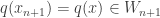
Let 


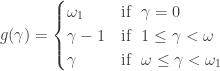
Now tweak the usual topology by calling sets of the form 

Note that any usual open interval 
Let 


Pictures of Continuous Functions
Consider the following two continuous functions.

Figure 1 – CDF of the standard normal distribution

Figure 2 – CDF of the uniform distribution
The first one (Figure 1) is the cumulative distribution function (CDF) of the standard normal distribution. The second one (Figure 2) is the CDF of the uniform distribution on the interval 

Consider a function that is continuous in the Sorgenfrey line but not continuous in the usual topology.

Figure 3 – Right continuous function
Figure 3 is a function that maps the interval 


The cumulative distribution function of a discrete probability distribution is always right continuous, hence continuous in the Sorgenfrey line. Here’s an example.

Figure 4 – CDF of a discrete uniform distribution
Figure 4 is the CDF of the uniform distribution on the finite set 
The take away from the last four figures is that the real-valued continuous functions defined on the Sorgenfrey line are right continuous and that step functions (with the left point solid and the right point hollow) are Sorgenfrey continuous.
A Family of Sorgenfrey Continuous Functions
The four examples of continuous functions shown above are excellent examples to illustrate the Sorgenfrey topology. We now introduce a family of continuous functions 

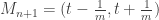
For any 
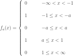

Figure 5 – a family of Sorgenfrey continuous functions
Function Space on the Sorgenfrey Line
This is the place where we switch the focus to function space. The set 

For the present discussion, all we need is some notation on a base for 
![[x,(a,b)]=\left\{h \in C_p(\mathbb{S}): h(x) \in (a, b) \right\}](https://s0.wp.com/latex.php?latex=%5Bx%2C%28a%2Cb%29%5D%3D%5Cleft%5C%7Bh+%5Cin+C_p%28%5Cmathbb%7BS%7D%29%3A+h%28x%29+%5Cin+%28a%2C+b%29+%5Cright%5C%7D&bg=ffffff&fg=333333&s=0&c=20201002)
![[x,(a,b)]](https://s0.wp.com/latex.php?latex=%5Bx%2C%28a%2Cb%29%5D&bg=ffffff&fg=333333&s=0&c=20201002)
The following is the main fact we wish to establish.
The function space 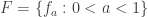
The above result will derive several facts on the function space
I invite readers to either verify the fact independently of the proof given here or follow the proof closely. Lots of drawing of the functions
Working out the Proof
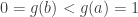
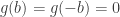
The following diagram was helpful to me as I worked out the different cases in showing the discreteness of the family

Figure 6 – A comparison of three Sorgenfrey continuous functions
Now the proof. First, 


![O=[a,V_1] \cap [-a,V_2]](https://s0.wp.com/latex.php?latex=O%3D%5Ba%2CV_1%5D+%5Ccap+%5B-a%2CV_2%5D&bg=ffffff&fg=333333&s=0&c=20201002)


The open set 


Now we show that
-
for each
 , there is an open set
  containing
  such that contains at most one point of .
Actually, this has already been done above with points 
Case 1. There exists some 

We assume that 


![U=[a,(-0.1,0.1)] \cap [-a,(0.9,1.1)]](https://s0.wp.com/latex.php?latex=U%3D%5Ba%2C%28-0.1%2C0.1%29%5D+%5Ccap+%5B-a%2C%280.9%2C1.1%29%5D&bg=ffffff&fg=333333&s=0&c=20201002)


Case 2. For every 
Claim. The function 


It follows that 


Now suppose we have 


It follows that 


The claim that the function ![U=[0,(0.9,1.1)]](https://s0.wp.com/latex.php?latex=U%3D%5B0%2C%280.9%2C1.1%29%5D&bg=ffffff&fg=333333&s=0&c=20201002)

![U=[-1,(-0.1,0.1)]](https://s0.wp.com/latex.php?latex=U%3D%5B-1%2C%28-0.1%2C0.1%29%5D&bg=ffffff&fg=333333&s=0&c=20201002)
We have established that the set
What does it Mean?
The above argument shows that the set
| Three Results |
|
To show that 


Secondly,
Thirdly,
Remarks
The topology of the Sorgenfrey line is vastly different from the usual topology on the real line even though the the Sorgenfrey topology is obtained by a seemingly small tweak from the usual topology. The real line is a metric space while the Sorgenfrey line is not metrizable. The real number line is connected while the Sorgenfrey line is not. The countable power of the real number line is a metric space and thus a normal space. On the other hand, the Sorgenfrey line is a classic example of a normal space whose square is not normal. See here for a basic discussion of the Sorgenfrey line.
The pictures of Sorgenfrey continuous functions demonstrated here show that the real number line and the Sorgenfrey line are also very different from a function space perspective. The function space
Though separable, the function space
For more information about
The next post is a continuation on the theme of drawing Sorgenfrey continuous functions.
Reference
- Arkhangelskii, A. V., Topological Function Spaces, Mathematics and Its Applications Series, Kluwer Academic Publishers, Dordrecht, 1992.
- Tkachuk V. V., A
-Theory Problem Book, Topological and Function Spaces, Springer, New York, 2011.


Normality in Cp(X)
Any collectionwise normal space is a normal space. Any perfectly normal space is a hereditarily normal space. In general these two implications are not reversible. In function spaces
Since we are discussing function spaces, the domain space
Let 
When Function Spaces are Normal
Let
- If the function space
- If the function space
- If the function space
- Let
Fact #1 and Fact #2 rely on a representation of 

Another useful tool is Dowker’s theorem, which essentially states that for any normal space 

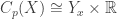
![W \times [0,1]](https://s0.wp.com/latex.php?latex=W+%5Ctimes+%5B0%2C1%5D&bg=ffffff&fg=333333&s=0&c=20201002)
To show Fact #1, suppose that 
![Y_x \times [0,1]](https://s0.wp.com/latex.php?latex=Y_x+%5Ctimes+%5B0%2C1%5D&bg=ffffff&fg=333333&s=0&c=20201002)

One more helpful tool is Theorem 5 in in this previous post, which is like an extension of Dowker’s theorem, which states that a normal space 


We want to show ![(Y_x \times \mathbb{R}) \times [0,1]](https://s0.wp.com/latex.php?latex=%28Y_x+%5Ctimes+%5Cmathbb%7BR%7D%29+%5Ctimes+%5B0%2C1%5D&bg=ffffff&fg=333333&s=0&c=20201002)
For Fact #2, a helpful tool is Katetov’s theorem (stated and proved here), which states that for any hereditarily normal 
To show Fact #2, suppose that
The proof of Fact #3 is found in Problems 294 and 295 of [2]. The key to the proof is a theorem by Reznichenko, which states that any dense convex normal subspace of ![[0,1]^X](https://s0.wp.com/latex.php?latex=%5B0%2C1%5D%5EX&bg=ffffff&fg=333333&s=0&c=20201002)
Fact #4 says that normality of the function space imposes countable extent on the domain. This result is discussed in this previous post (see Corollary 3 and Corollary 5).
Remarks
The facts discussed here give a flavor of what function spaces are like when they are normal spaces. For further and deeper results, see [1] and [2].
Fact #1 is essentially driven by Dowker’s theorem. It follows from the theorem that whenever the product space 

The driving force behind Fact #2 is Katetov’s theorem, which basically says that the hereditarily normality of
There are examples of normal but not collectionwise normal spaces (e.g. Bing’s Example G). Resolution of the question of whether normal but not collectionwise normal Moore space exists took extensive research that spanned decades in the 20th century (the normal Moore space conjecture). The function
On the other hand, a more interesting point is on the normality of
Reference
- Arkhangelskii, A. V., Topological Function Spaces, Mathematics and Its Applications Series, Kluwer Academic Publishers, Dordrecht, 1992.
- Tkachuk V. V., A
Looking for spaces in which every compact subspace is metrizable
Once it is known that a topological space is not metrizable, it is natural to ask, from a metrizability standpoint, which subspaces are metrizable, e.g. whether every compact subspace is metrizable. This post discusses several classes of spaces in which every compact subspace is metrizable. Though the goal here is not to find a complete characterization of such spaces, this post discusses several classes of spaces and various examples that have this property. The effort brings together many interesting basic and well known facts. Thus the notion “every compact subspace is metrizable” is an excellent learning opportunity.
Several Classes of Spaces
The notion “every compact subspace is metrizable” is a very broad class of spaces. It includes well known spaces such as Sorgenfrey line, Michael line and the first uncountable ordinal 
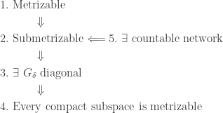
Let 


Let 


The diagonal of the space 


The implication 


None of the implications in the diagram is reversible. The first uncountable ordinal 


To see where the examples mentioned earlier are placed, note that Sorgenfrey line and Michael line are submetrizable, both are submetrizable by the usual Euclidean topology on the real line. Each compact subspace of the space ![[0,\alpha]](https://s0.wp.com/latex.php?latex=%5B0%2C%5Calpha%5D&bg=ffffff&fg=333333&s=0&c=20201002)
Function Spaces
We now look at some function spaces that are in the class “every compact subspace is metrizable.” For any Tychonoff space (completely regular space)
Theorem 1
Suppose that
Proof
The proof here actually shows more than is stated in the theorem. We show that 


Let 


We claim that 
For 


Theorem 1 is actually a special case of a duality result in
Corollary 2
Let 


The key fact for Corollary 2 is that the product of continuum many separable spaces is separable (this fact is discussed here). Theorem 1 is actually a special case of a deep result.
Theorem 3
Suppose that 

Theorem 3 is a much more general result. The product of any arbitrary number of separable spaces is not separable if the number of factors is greater than continuum. So the proof for Theorem 1 will not work in the general case. This result is Problem 307 in [2].
A Duality Result
Theorem 1 is stated in a way that gives the right information for the purpose at hand. A more correct statement of Theorem 1 is:
The cardinal function of density is the least cardinality of a dense subspace. For any space 

There is a duality result between density and weak weight for
The density of
Reference
- Arkhangelskii, A. V., Topological Function Spaces, Mathematics and Its Applications Series, Kluwer Academic Publishers, Dordrecht, 1992.
- Tkachuk V. V., A
Comparing two function spaces
Let 


____________________________________________________________________
Tightness
One topological property that is different between
Let 


First, we show that the tightness of 


The space
Theorem 1
Let 

Theorem 1 is a special case of Theorem I.4.1 on page 33 of [1] (the countable case). One direction of Theorem 1 is proved in this previous post, the direction that will give us the desired result for
____________________________________________________________________
The Frechet-Urysohn property
In fact,
____________________________________________________________________
Normality
The function space
____________________________________________________________________
Embedding one function space into the other
The two function space 


The homeomposhism
On the other hand, the function space
____________________________________________________________________
Remark
There is a mapping that is alluded to at the beginning of the post. Each 
____________________________________________________________________
Reference
- Arkhangelskii, A. V., Topological Function Spaces, Mathematics and Its Applications Series, Kluwer Academic Publishers, Dordrecht, 1992.
- Buzyakova, R. Z., In search of Lindelof
____________________________________________________________________

Cp(omega 1 + 1) is monolithic and Frechet-Urysohn
This is another post that discusses what
____________________________________________________________________
Initial discussion
The function space 

The subspace 

____________________________________________________________________
Connection to
We show that the function space 

Every function in
By Theorem 1 in this previous post, 


Thus
____________________________________________________________________
A closer look at
In fact 


Clearly 


____________________________________________________________________
Monolithicity and Frechet-Urysohn property
As indicated at the beginning, the
Let 

A space 

In any monolithic space, the density and the network weight coincide for any subspace, and in particular, any subspace that is separable has a countable network. As a result, any separable monolithic space has a countable network. Thus any separable space with no countable network is not monolithic, e.g., the Sorgenfrey line. On the other hand, any space that has a countable network is monolithic.
In any strongly monolithic space, the density and the weight coincide for any subspace, and in particular any separable subspace is metrizable. Thus being separable is an indicator of metrizability among the subspaces of a strongly monolithic space. As a result, any separable strongly monolithic space is metrizable. Any separable space that is not metrizable is not strongly monolithic. Thus any non-metrizable space that has a countable network is an example of a monolithic space that is not strongly monolithic, e.g., the function space ![C_p([0,1])](https://s0.wp.com/latex.php?latex=C_p%28%5B0%2C1%5D%29&bg=ffffff&fg=333333&s=0&c=20201002)
The function space
For any compact space 


____________________________________________________________________
General discussion
For any compact space
Theorem 1
Then the function space
See chapter 3 section 6 of [1] for a discussion of stable spaces. We give the definition here. A space 


All compact spaces are stable. Let 


Corollary 2
Let
However, the strong monolithicity of
Theorem 3
Let
A space 
![[0,1]](https://s0.wp.com/latex.php?latex=%5B0%2C1%5D&bg=ffffff&fg=333333&s=0&c=20201002)
For compact spaces
Theorem 4
Let
- The compact space
A space
____________________________________________________________________
Reference
- Arkhangelskii, A. V., Topological Function Spaces, Mathematics and Its Applications Series, Kluwer Academic Publishers, Dordrecht, 1992.
____________________________________________________________________
A useful representation of Cp(X)
Let
Theorem 1
Let

Then 
The above theorem can be found in [1] (see Theorem I.5.4 on p. 37). In [1], the homeomorphism is stated without proof. For the sake of completeness, we provide a detailed proof of Theorem 1.
Proof of Theorem 1
Define 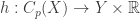

The map is one-to-one
First, we show that it is a one-to-one map. Let 


The map is onto
Now we show 


Note. Showing the continuity of 
The map is continuous
Show that 


where 


Then define the open set

Clearly 


Subtracting the above two inequalities, we have the following:

The above inequality shows that for each 
The inverse is continuous
We now show that 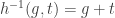


where 


We need to show that 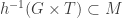

Adding the above two inequalities, we obtain:

The above implies that 


____________________________________________________________________
Reference
- Arkhangelskii, A. V., Topological Function Spaces, Mathematics and Its Applications Series, Kluwer Academic Publishers, Dordrecht, 1992.
____________________________________________________________________
A useful embedding for Cp(X)
Let
Theorem 1
Suppose that the space
Proof of Theorem 1
Let 


First we show 


Next we show that 

where 


Clearly 


Now we show that 


where 


Clearly 


____________________________________________________________________
Example
The proof of Theorem 1 is not difficult. It is a matter of notating carefully the open sets in both function spaces. However, the embedding makes it easy in some cases to understand certain function spaces and in some cases to relate certain function spaces.
Let 
The map
____________________________________________________________________
Cp(X) is countably tight when X is compact
Let 
____________________________________________________________________
Tightness
Let
The fact that
Theorem 1
Let
Theorem 1 is the countable case of Theorem I.4.1 on page 33 of [1]. We prove one direction of Theorem 1, the direction that will give us the desired result for
Proof of Theorem 1
The direction
Suppose that 


Let 


For each 


We now show that 

 .
.
We wish to show that 


The direction
See Theorem I.4.1 of [1].

____________________________________________________________________
Remarks
As shown above, countably tightness is one convergence property of
____________________________________________________________________
Reference
- Arkhangelskii, A. V., Topological Function Spaces, Mathematics and Its Applications Series, Kluwer Academic Publishers, Dordrecht, 1992.
____________________________________________________________________

Cp(omega 1 + 1) is not normal
In this and subsequent posts, we consider
Let
For the basic working of function spaces with the pointwise convergence topology, see the post called Working with the function space Cp(X).
The fact that
- If
- There exists an uncountable closed and discrete subspace of
.
We discuss each of the bullet points separately.
The function space
Now we show that there exists an uncountable closed and discrete subspace of 

Clearly, 
Let 
Claim 1
There exists an open subset 

Consider the two mutually exclusive cases. Case 1. There exists some 
For Case 1, let 
Now assume Case 2. Within this case, there are three sub cases. Case 2.1.
Case 2.1. If 


Case 2.2. Suppose 
Case 2.3. Suppose 

Case 2.3.1. Just like in Case 2.2, let
Case 2.3.2. Assume that 


Case 2.3.2.1. Define 
Case 2.3.2.2. In this case, 


In all the cases except the last one, Claim 1 is true. The last case is not possible. Thus Claim 1 is established. The set
Next we show that 


We have established that
Remarks
The set
Because 


The function space 
Is 

It seems that the argument above for showing
Reference
- Arhangel’skii, A. V., Normality and Dense Subspaces, Proc. Amer. Math. Soc., 48, no. 2, 283-291, 2001.
- Baturov, D. P., Normality in dense subspaces of products, Topology Appl., 36, 111-116, 1990.
Revised 9/17/2018
The canonical evaluation map with a function space perspective
The evaluation map is a useful tool for embedding a space into a product space and plays an important role in many theorems and problems in topology. See here for a previous discussion. In this post, we present the evaluation map with the perspective that the map can be used for embedding a space into a function space of continuous functions. This post will be useful background for subsequent posts on
____________________________________________________________________
The general setting
Let 


One more comment before defining the evaluation map. The set 

We now define the evaluation map. Define the map 


The map 

____________________________________________________________________
What makes the evaluation map works
The goal of the evaluation map is that it be a homeomorphism. For that to happen, we need to make a few more additional assumptions. In defining the evaluation map above, the functions in the family 
Theorem 1
Let
Proof of Theorem 1
Let 

where 


In order to make the evaluation map a homeomorphism, we consider two more definitions. A family 


Theorem 2
Let
- If
- If
Proof of Theorem 2
To prove the bullet point 1, suppose that 
To prove the bullet point 2, suppose that the family 


Clearly 


____________________________________________________________________
Embedding every space into a function space
In defining the evaluation map, we start with a space 
Corollary 3a
Any space 
Because 

![I=[0,1]](https://s0.wp.com/latex.php?latex=I%3D%5B0%2C1%5D&bg=ffffff&fg=333333&s=0&c=20201002)
Corollary 3b
Any space 
We can also let 

Corollary 3c
Any space 
____________________________________________________________________
One application
We demonstrate one application of Corollary 3a. When
Theorem 4
Let
- The space
- The space
Proof of Theorem 4
The direction 

Suppose that 
![[M,V]](https://s0.wp.com/latex.php?latex=%5BM%2CV%5D&bg=ffffff&fg=333333&s=0&c=20201002)


Any space with a countable network is the continuous image of a separable metric space. Thus there exists a separable metric space 

By Corollary 3a,
____________________________________________________________________
More on the evaluation map
In this section, we consider some special cases. As shown in Theorem 2, what makes the evaluation map a one-to-one map is that the family
The family

Since 
Theorem 5
Let
We now show that if
First one definition. Let 


Lemma 6
Let the space
Proof of Lemma 6
Let 

where 


Let 


Corollary 7
Let the space
In Corollary 7, even if 
Corollary 8
If
____________________________________________________________________
Reference
- Arkhangelskii, A. V., Topological Function Spaces, Mathematics and Its Applications Series, Kluwer Academic Publishers, Dordrecht, 1992.
____________________________________________________________________
