Paracompact spaces and Lindelof spaces are familiar notions of covering properties. The covering properties resulting from replacing the para with meta in the case of paracompact and adding meta to Lindelof are also spaces that had been extensively studied. This is an introduction of meta-Lindelof spaces by way of examples.
Definitions
All spaces under discussion are Hausdorff and regular. A space  is paracompact if every open cover of has a locally finite open refinement. A space is metacompact if every open cover of has a point-finite open refinement. A space is Lindelof if every open cover of has a countable subcover, i.e., every open cover of has a countable subcollection that is also a cover of . A space is meta-Lindelof if every open cover of has a point-countable open refinement, i.e., every open cover
  of has a subcollection
  such that is a refinement of and that is a point-countable collection. From the definitions, we have the implications shown in the following diagram.
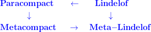
It is well known that any regular Lindelof space is paracompact (the left arrow at the top of the diagram). The two down arrows and the right arrow at the bottom in the diagram follow from the definitions. If there is an up arrow from meta-Lindelof to Lindelof, the diagram would be a closed loop, which would mean all 4 notions are equivalent. At minimum, there are paramcompact spaces that are not Lindelof. For example, any non-separable metric space is paracompact and not Lindelof. Thus, in general it is impossible for the diagram to be a closed loop. In other words, there must be meta-Lindelof spaces that are not Lindelof. However, with additional assumptions, an up arrow from meta-Lindelof to Lindelof is possible. Theorem 1 below shows that the diagram is a closed loop for separable spaces. It is well known that paracompact spaces with the countable chain condition (CCC) are Lindelof (see here). Perhaps an up arrow from meta-Lindelof to Lindelof is possible for spaces with CCC. We discuss some partial results at the end of this article.
Spaces that are not meta-Lindelof
We present two spaces that are not meta-Lindelof (Example 1 and Example 2). The following theorem will make the examples clear.
Theorem 1
Let be a separable space. If is meta-Lindelof, then is Lindelof.
Proof
Let be an open cover of . Since is meta-Lindelof, there is a point-countable open refinement of . Let  be a countable dense subset of . Let
  be defined by
  . Since is point-countable, each point of can belong to only countably many
  . It follows that is countable. Furthermore,
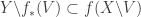
  . The set inclusion
  is clear. The set inclusion
  follows from the fact that is a dense subset. To complete the proof, for each
  , choose
  such that
  . Then
  is a countable subcover of . This completes the proof that is Lindelof.
In the above proof, the countable dense set forces the point-countable open refinement to be countable, thus leading to a countable subcover of the original open cover. We now look at examples.
Example 1
The idea for this example is that any separable space that is known to be non-Lindelof must not be meta-Lindelof due to the above theorem. A handy example is the Sorgenfrey plane  . Recall that the Sorgenfrey line
  is the real number line topologized by the base consisting of the half open intervals of the form
  . It is well known that is hereditarily Lindelof, separable and not metrizable. The Sorgenfrey line is a classic example of a Lindelof space whose square is not even normal, thus not Lindelof (see here). By Theorem 1, the Sorgenfrey plane is not meta-Lindelof.
Example 2
This is another example that is separable and non-Lindelof, hence not meta-Lindelof. The space is the Mrowka space (or Psi-space), which is defined here. To define the space, let  be uncountable almost disjoint family of subsets of
  , that is, for any
  with
with  ,
,  is finite. The underlying set is
  . The points in are isolated. An open neighborhood of
  is of the form
  where
where  is a finite set. The space is not Lindelof since is an uncountable closed and discrete subset. It is separable since the set of integers, , is a dense subset. By Theorem 1, the space must not be meta-Lindelof. This space is a classic example of a space that has a
  -diagonal but is not submetrizable.
Example 3
Example 1 is not normal. Example 2 is not normal if the almost disjoint family has cardinality continuum (due to Jones’ Lemma). For Example 2 to be normal, additional set theory axiom is required. Example 3 is a normal example of a space that is not meta-Lindelof.
Consider  , the space of the countable ordinals with the ordered topology. This space is not Lindelof since the open cover consisting of
 ![[0,\alpha]](https://s0.wp.com/latex.php?latex=%5B0%2C%5Calpha%5D&bg=ffffff&fg=333333&s=0&c=20201002) , where
, where  , is an open cover that has no countable subcover. The space is also not paracompact since some open covers cannot be locally finite. The same idea can show that certain open covers cannot be point-countable open cover. This is due to the pressing down lemma (see here). To see this, for each limit ordinal , let
 ![O_\alpha=(f(\alpha), \alpha]](https://s0.wp.com/latex.php?latex=O_%5Calpha%3D%28f%28%5Calpha%29%2C+%5Calpha%5D&bg=ffffff&fg=333333&s=0&c=20201002) be an open set containing
be an open set containing  . Then the function
  is a so called pressing down function. By the pressing down lemma, there exist some
  such that the set
  is a stationary subset of . This implies that the point would belong to uncountably many open sets
  . Thus, any open cover of containing the sets cannot be point-countable.
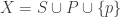
To wrap up the example, let be any open refinement of the open cover consisting of the open sets ![[0, \alpha]](https://s0.wp.com/latex.php?latex=%5B0%2C+%5Calpha%5D&bg=ffffff&fg=333333&s=0&c=20201002) . We choose described above such that each is contained in some
. We choose described above such that each is contained in some  . This means that cannot be point-countable. Thus, one open cover of has no point-countable open refinement, showing that the space of all countable ordinals,
  , cannot be meta-Lindelof.
Example 4
This example makes use of Example 3. Consider be the product space of many copies of the real line  . Each
  is a function
  . Let
. Let  denote
  for each . Let
  be the set of all points
  in where is non-zero for at most countably many . This space is called the
  -product of lines. The topology of is the inherited product topology from the product space . The -product of separable metric spaces is collectionwise normal (see here). The -product of uncountably many spaces, each of which has at least 2 points, always contains a closed copy of the space (see here).
Observe that closed subspaces of a meta-Lindelof space are always meta-Lindelof. Thus the -product defined here cannot be a meta-Lindelof space. This example is revisited in Example 6 below.
Meta-Lindelof but not Lindelof
Example 5
This example is the Michael line  , which is the real line topologized by making the irrational numbers isolated and letting the rational numbers retain the usual Euclidean open sets (a basic introduction is found here). The usual Euclidean open sets of the real line are also open in the Michael line. Thus, is a submetrizable space.
To see that it is meta-Lindelof, let be an open cover of the Michael line . Choose  such that
  covers the rational numbers. Let
  . Thus is a point-countable open refinement of . This shows that the Michael line is meta-Lindelof. This fact can also be seen from the above diagram, which shows that paracompact
  metacompact meta-Lindelof. Note that the Michael line is a paracompact space that is not Lindelof.
The Michael line as an example of a meta-Lindelof space is quite informative. Note that in any Lindelof space, all closed and discrete subsets must be countable (such a space is said to have countable extent). However, a meta-Lindelof space can have uncountable closed and discrete subset. There is a closed and discrete subset of the Michael line of cardinality continuum. To see this, note that there is a Cantor set in the real line consisting entirely of irrational numbers. For example, we can construct a Cantor set within the interval ![A=[\sqrt{2},\sqrt{8}]](https://s0.wp.com/latex.php?latex=A%3D%5B%5Csqrt%7B2%7D%2C%5Csqrt%7B8%7D%5D&bg=ffffff&fg=333333&s=0&c=20201002) . Let
. Let  enumerate all rational numbers within this interval. In the first step, we remove a middle part of the interval such that the two remaining closed intervals have irrational endpoints and will miss
  . In the
  th step of the construction, we remove the middle part of each of the remaining intervals such that all remaining intervals have irrational endpoints and will miss the rational number
  . Let
. Let  be the resulting Cantor set, which consists only of irrational numbers since it misses all rational numbers in . The set , as a subset of the Michael line, is closed and discrete.
The above paragraph shows one direction in which the two notions of “Lindelof” diverge. Lindelof spaces have countable extent. On the other hand, meta-Lindelof space can have uncountable closed and discrete subsets.
Example 5 actually presents a template for producing meta-Lindelof spaces. In Example 5, start with the real line with the usual topology. Identify a “Lindelof” part (the rationals) and make the remainder discrete (the irrationals). The template is further described in the following theorem.
Theorem 2
Let be a space and let  be a Lindelof subspace of . Define a new space
  such that the underlying set is and the new topology is defined as follows. Let points
  be isolated and let points
  retain the original open sets in .
- Then the space is a meta-Lindelof space.
- If the original space is a non-Lindelof space, then is also not Lindelof.
To see with the new topology is meta-Lindelof, follow the same proof in showing the Michael line is meta-Lindelof. To prove part 2, let be an open cover of (in the original topology) such that no countable subcollection of is a cover of . Let  be a countable subcollection of such that covers . There must be uncountably many points of not covered by . Then
  is an open cover of that has no countable subcover.
Example 6
This example starts with the space in Example 4. To define , let  , the product space of many copies of the real line . Let and be the subspaces of defined as follows:
The space is called the -product of lines and is collectionwise normal. Note that the -product of separable metric spaces is collectionwise normal (see here). The space is called the  -product of lines, which consists of all points in the product space with non-zero values in at most finitely many coordinates. Note that the -product of separable metric spaces is a Lindelof space (see here).
The -product is not Lindelof because it contains a closed copy of (see here). Thus, is a non-Lindelof space with a Lindelof subspace , which is exactly what is required in Theorem 2. Define the space as described in Theorem 2. The resulting is meta-Lindelof but not Lindelof.
Note that the Lindelof is a dense subset of -product . Thus, though is not Lindelof, it has a dense Lindelof subspace. In Example 4, we see that is not meta-Lindelof since it contains a non-meta-Lindelof space as a closed subspace. However, re-topologizing it by making the points not in isolated and making the points in retain the open sets in the -product topology produces a meta-Lindelof space.
Concluding Remarks
A few observations can be made from the six examples discussed above.
- Among the separable spaces, meta-Lindelofness and Lindelofness are the same (Theorem 1). This gives a handy way to show that any separable space that is not Lindelof is not meta-Lindelof.
- It is possible that the product of Lindelof spaces is not meta-Lindelof (Example 1).
- A question can be asked for Example 2, which is a Moore space. Any Lindelof Morre space is second countable. Example 2 is not meta-Lindelof. Must a meta-Lindelof Moore space be second countable?
- The first uncountable ordinal with the order topology is not paracompact since it is not possible to cover the limit ordinals with a locally finite collection of open sets. The same idea shows that does not even satisfy the weaker property of meta-Lindelof (Example 3).
- One take away from Example 4 is that meta-Lindelof spaces resemble Lindelof spaces in one respect, that is, meta-Lindelofness is hereditary with respect to closed subspaces. Because the -product of the real lines contains a closed copy of , it is not meta-Lindelof.
- The Michael line (Example 5) demonstrates one critical difference between meta-Lindelof and Lindelof. Any Lindelof space has countable extent. It is different for meta-Lindelof spaces. In the Michael line, there is an uncountable closed and discrete subset. One way to see this is to construct a Cantor set in the real line consisting of only irrational numbers.
- The Michael line (Example 5) gives the hint of a recipe for producing meta-Lindelof spaces. The recipe is described in Theorem 2. Example 6 is a demonstration of the recipe. The -product discussed inExample 4 is non-Lindelof with a dense Lindelof subspace . By letting retain the original -product open sets and making the complement of discrete, we produce another meta-Lindelof space that is not Lindelof.
The rest of the remark focuses on the diagram given earlier (repeated belo
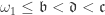
Theorem 1 shows that for separable spaces, meta-Lindelof Lindelof. As a result, the diagram becomes a closed loop, meaning all 4 notions in the diagram are equivalent for separable spaces. As pointed out earlier, CCC may be a good candidate for replacing separable since among CCC spaces, paracompactness equates Lindelofness. It turns out that for CCC spaces, meta-Lindelof does not imply Lindelof. A handy example is the Pixley-Roy space ![\mathcal{F}[\mathbb{R}]](https://s0.wp.com/latex.php?latex=%5Cmathcal%7BF%7D%5B%5Cmathbb%7BR%7D%5D&bg=ffffff&fg=333333&s=0&c=20201002) , which is non-Lindelof, metacompact (hence meta-Lindelof) and satisfies the CCC (see the follow up discussion in the next post). We found the following partial result in p. 971 of the Handbook of Set-Theoretic Topology (Chapter 22 on Borel Measures by Gardner and Pfeffer).
, which is non-Lindelof, metacompact (hence meta-Lindelof) and satisfies the CCC (see the follow up discussion in the next post). We found the following partial result in p. 971 of the Handbook of Set-Theoretic Topology (Chapter 22 on Borel Measures by Gardner and Pfeffer).
Theorem 3 (MA + not CH)
Each locally compact meta-Lindelof space satisfying the CCC is Lindelof.
Theorem 3 is Corollary 4.9 in the article in the Handbook. It implies that for locally compact CCC space, the above diagram is a closed loop but only under Martin’s axiom and the negation of CH.
The Handbook was published in 1984. We wonder if there is any update since then. For any reader who has updated information regarding the consistency result in Theorem 3, please kindly comment in the space below.
For more information on meta-Lindelof and other covering properties, see Chapter 9 in the Handbook of Set-Theoretic Topology (the chapter by D. Burke on covering properties).

Dan Ma topology
Daniel Ma topology
Dan Ma Lindelof spaces
Daniel Ma Lindelof spaces
Dan Ma meta-Lindelof spaces
Daniel Ma meta-Lindelof spaces
 2022 – Dan Ma
Posted: 10/29/2022
Updated: 10/30/2022
Updated: 11/1/2022


is made an isolated point.
 where
where 


 be a quotient map. Let the map
  be defined by
  for each
  . Then the map
  to
to  .
. and
and  ,
,  is an open set in
  is an open set in
  . We proceed to find some open set
  such that
  .
. and an open set
  with
with  such that
  is compact and
  . We make the following observation,
 ,
,  if and only if
 . By observation (1), we have
  . Note that
  . Thus,
  . As a result, we have
  is open in
 be the projection map. Since
  is a closed map according to the Kuratowski Theorem (see
  is closed in
  ,
,  is closed in
  is open in
  . Thus,
  such that
  be a quotient map from
  defined by
  . By Theorem 1,
  , we establish that
  be a quotient map from
  by letting
  . According to Theorem 1,
  , we establish that
  such that each
  is isolated and an open neighborhood of
  with the usual Euclidean topology. Let
  be the topological sum of
  , which is called a spine.
 is always a sequential space. According to Corollary 4,
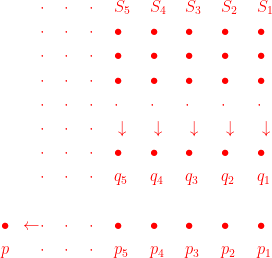
 . In this Euclidean space, the points in the sequences
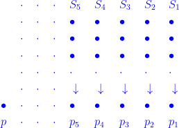
 with the quotient topology. With the quotient topology, an open set containing the point
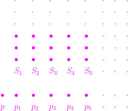
 consists of the point
  . Note that no sequence of points in
  . As observed in the preceding paragraph, no sequence of points in
  be a mapping from a topological space
  if the following holds: for any mapping
  , is a closed map if for any closed subset
  is closed in
  is compact for each
  be a closed map with
  . Then the set
  is open in
  .
. , define
  . By Lemma 3, each
  is an open subset of
  is an open cover of
  such that
  . Since
  . It follows that
  . Since
  such that
  . For each
  for some
  . We claim that
  is a cover of
  . This implies that
  . Thus, the open cover
  .
. . (1) It is an open cover of
  such that
  and such that
  such that
  and such that
  intersects only finitely many elements of
  . Let
. Let  . Clearly,
  ,
, ,
, . To see (3), let
  where
where  . Then
  for some
  . Let
. Let  . Then
  . This implies that
  . It follows that
  , i.e., the weight of
  be a map (or function) from
  is closed in
  be open. Let
  is closed in
  . Note that
  is closed in
 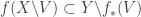 . Let
. Let  . Then
  for some
  . Since
  and
and  , we have
  . This implies that
  .
. . Let
. Let  . Since
  ,
,  . Choose
  , which implies that
  .
. . We have
  . As a result,
  for some
  .
.  be a base for
  for
for  , i.e., the cardinality of
  is a base for
  is defined in Lemma 2. Let
  be an open set. Let
  . For each
  , choose
  such that
  and
and  . Since
  such that
  . Note that
  . Since
  , we have
  . We also have
  . Thus, every open subset
  of
of  would be a base for
  be the real line with the usual topology. Collapse the closed interval
 ![[1,2]](https://s0.wp.com/latex.php?latex=%5B1%2C2%5D&bg=ffffff&fg=333333&s=0&c=20201002) to one point called
to one point called  . In
. In  are the usual Euclidean neighborhoods. The open neighborhoods of the point
  ,
,  , which is not open in
  ,
,  , which is not open in
  ,
,  may not be open but has an open subset
  be a property of topological spaces. We say that
  , if the space
  ” is an invariant of the perfect maps.
 -space.
 such that
  . A network behaves like a base but the elements of the network do not have to be open sets. Of interest are the spaces with a countable network. Compact spaces with a countable network is metrizable. Any space with a countable network is both hereditarily separable and hereditarily Lindelof. The space
  with
with  . Let
. Let  be the x-axis, which is the set of all pairs of real numbers
  . The bow-tie space is the set
  with the topology defined as follows.
 with
with  . Each set
  having Euclidean distance less than
  from
from  , respectively.
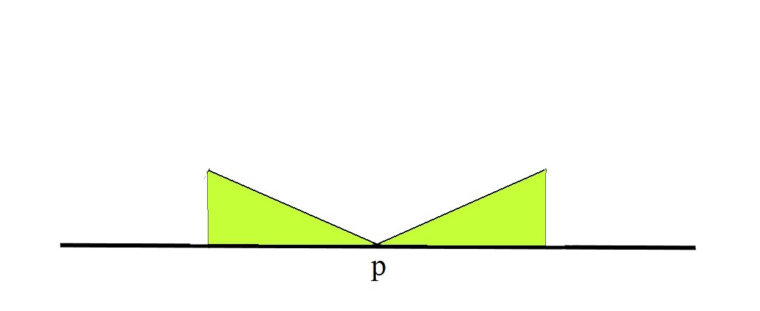
 be countable bases for
  is a network for the Bow-Tie space
  be the upper half plane
  be the x-axis
  , the free sum or free union. This means that
  is open if and only if both
  and
and  are open. It follows that the identity map from
  onto the Bow-Tie space
  ,
,  ,
,  ,
,  . Pick
  such that
  for all
  . Consider
  . Since
  . This means that both the left side and the right side of the bow-tie in
  are within
  , the function space with the pointwise convergence topology on the Bow-Tie space
  is a Lindelof
  is a hereditarily D-space.
 from the space
  is a closed map.
 where
where  with
with  , which is not closed in
  is clear. We prove
  and
and  .
. is open in
  . Note that
  . By the Tube Lemma (see
  . It follows that
  . This means that
  is closed in
  (see
(see  . Let
. Let  . Define a topology on
 are of the form
  where
where  is finite and
  . In words, we can describe the topology on
  . the intersection of finitely many sets in
  for some
  . As a result,
  and
and  are disjoint open sets separating
  and
and  be disjoint closed subsets of
  and
and  where
where  . By assumption,
  is closed in
  . Since
  , we have
  . This means that
  . Furthermore, there exists
  such that
  . We claim that
  for all
  . Consider the open set
  , which contains the point
  . Since
  , the open set
  . Thus
  for some
  . This means that
  and
and  . What we have just shown is that for every open set
  ,
,  for all
  , which is compact. Thus, each point inverse of the projection map is compact.
 ![\mathcal{F}[X]](https://s0.wp.com/latex.php?latex=%5Cmathcal%7BF%7D%5BX%5D&bg=ffffff&fg=333333&s=0&c=20201002) , which is always metacompact, hence meta-Lindelof. We then make sure the ground
, which is always metacompact, hence meta-Lindelof. We then make sure the ground ![F \in \mathcal{F}[X]](https://s0.wp.com/latex.php?latex=F+%5Cin+%5Cmathcal%7BF%7D%5BX%5D&bg=ffffff&fg=333333&s=0&c=20201002) and any open
and any open  , define
 ![[F,U]](https://s0.wp.com/latex.php?latex=%5BF%2CU%5D&bg=ffffff&fg=333333&s=0&c=20201002) as follows:
as follows:![[F,U]=\{ D \in \mathcal{F}[X]: F \subset D \subset U \}](https://s0.wp.com/latex.php?latex=%5BF%2CU%5D%3D%5C%7B+D+%5Cin+%5Cmathcal%7BF%7D%5BX%5D%3A+F+%5Csubset+D+%5Csubset+U+%5C%7D&bg=ffffff&fg=333333&s=0&c=20201002)
 such that
  . This sounds like the definition of a base for a topology. Note that the sets in the network
 ![\{ [F_\alpha,U_\alpha]: \alpha \in \omega_1 \}](https://s0.wp.com/latex.php?latex=%5C%7B+%5BF_%5Calpha%2CU_%5Calpha%5D%3A+%5Calpha+%5Cin+%5Comega_1+%5C%7D&bg=ffffff&fg=333333&s=0&c=20201002) be an uncountable collection of open sets in
be an uncountable collection of open sets in  such that
  . Since
  such that
  for uncountably many
  and
and  . Then we have
  and
and  . Note that the finite set
  belongs to both
 ![[F_\beta,U_\beta]](https://s0.wp.com/latex.php?latex=%5BF_%5Cbeta%2CU_%5Cbeta%5D&bg=ffffff&fg=333333&s=0&c=20201002) and
and ![[F_\gamma,U_\gamma]](https://s0.wp.com/latex.php?latex=%5BF_%5Cgamma%2CU_%5Cgamma%5D&bg=ffffff&fg=333333&s=0&c=20201002) . This completes the proof that the Pixley-Roy space
. This completes the proof that the Pixley-Roy space 

 , where
  be the listing of all the prime numbers. Suppose that
  converges. There is some positive integer
  such that
  . In the remainder of the proof, the prime numbers
  are called small primes and
  are called big primes. For any positive integer
  , we have the following inequality:
 be the number of all positive integers
  such that the prime divisors of
  be the number of all positive integers
  for all
  for some
  refers to the floor function, which is greatest integer less than or equal to
  , which is identical to the number of positive integers
  . We now have the following upper bound for
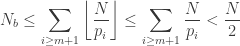
 is square-free while
  is not square-free. Note that any positive integer
  with
with  being square-free. If a positive integer is itself square-free, the square part is 1. Otherwise, we can always rearrange the prime decomposition to obtain
  where
where  is square-free part. Each
  many different square-free parts
  , we have
  . The following is an upper bound on
 or
or  . A good choice is
  . With this particular
 , which contradicts the fact that
  , are there arithmetic progression of primes of length