Pseudocompact spaces with regular G-delta diagonals

Posted on February 19, 2018 by Dan Ma

This post complements two results discussed in two previous blog posts concerning $G_\delta$ -diagonal. One result is that any compact space with a $G_\delta$ -diagonal is metrizable (see here). The other result is that the compactness in the first result can be relaxed to countably compactness. Thus any countably compact space with a $G_\delta$ -diagonal is metrizable (see here). The countably compactness in the second result cannot be relaxed to pseudocompactness. The Mrowka space is a pseudocompact space with a $G_\delta$ -diagonal that is not submetrizable, hence not metrizable (see here). However, if we strengthen the $G_\delta$ -diagonal to a regular $G_\delta$ -diagonal while keeping pseudocompactness fixed, then we have a theorem. We prove the following theorem.

Theorem 1
If the space $X$ is pseudocompact and has a regular $G_\delta$ -diagonal, then $X$ is metrizable.

All spaces are assumed to be Hausdorff and completely regular. The assumption of completely regular is crucial. The proof of Theorem 1 relies on two lemmas concerning pseudocompact spaces (one proved in a previous post and one proved here). These two lemmas work only for completely regular spaces.

The proof of Theorem 1 uses a metrization theorem. The best metrization to use in this case is Moore metrization theorem (stated below). The result in Theorem 1 is found in [2].

First some basics. Let $X$ be a space. The diagonal of the space $X$ is the set $\Delta=\{ (x,x): x \in X \}$ . When the diagonal $\Delta$ , as a subset of $X \times X$ , is a $G_\delta$ -set, i.e. $\Delta$ is the intersection of countably many open subsets of $X \times X$ , the space $X$ is said to have a $G_\delta$ -diagonal.

The space $X$ is said to have a regular $G_\delta$ -diagonal if the diagonal $\Delta$ is a regular $G_\delta$ -set in $X \times X$ , i.e. $\Delta=\bigcap_{n=1}^\infty \overline{U_n}$ where each $U_n$ is an open subset of $X \times X$ with $\Delta \subset U_n$ . If $\Delta=\bigcap_{n=1}^\infty \overline{U_n}$ , then $\Delta=\bigcap_{n=1}^\infty \overline{U_n}=\bigcap_{n=1}^\infty U_n$ . Thus if a space has a regular $G_\delta$ -diagonal, it has a $G_\delta$ -diagonal. We will see that there exists a space with a $G_\delta$ -diagonal that fails to be a regular $G_\delta$ -diagonal.

The space $X$ is a pseudocompact space if for every continuous function $f:X \rightarrow \mathbb{R}$ , the image $f(X)$ is a bounded set in the real line $\mathbb{R}$ . Pseudocompact spaces are discussed in considerable details in this previous post. We will rely on results from this previous post to prove Theorem 1.

The following lemma is used in proving Theorem 1.

Lemma 2
Let $X$ be a pseudocompact space. Suppose that $O_1,O_2,O_2,\cdots$ is a decreasing sequence of non-empty open subsets of $X$ such that $\bigcap_{n=1}^\infty O_n=\bigcap_{n=1}^\infty \overline{O_n}=\{ x \}$ for some point $x \in X$ . Then $\{ O_n \}$ is a local base at the point $x$ .

Proof of Lemma 2
Let $O_1,O_2,O_2,\cdots$ be a decreasing sequence of open subsets of $X$ such that $\bigcap_{n=1}^\infty O_n=\bigcap_{n=1}^\infty \overline{O_n}=\{ x \}$ . Let $U$ be open in $X$ with $x \in U$ . If $O_n \subset U$ for some $n$ , then we are done. Suppose that $O_n \not \subset U$ for each $n$ .

Choose open $V$ with $x \in V \subset \overline{V} \subset U$ . Consider the sequence $\{ O_n \cap (X-\overline{V}) \}$ . This is a decreasing sequence of non-empty open subsets of $X$ . By Theorem 2 in this previous post, $\bigcap \overline{O_n \cap (X-\overline{V})} \ne \varnothing$ . Let $y$ be a point in this non-empty set. Note that $y \in \bigcap_{n=1}^\infty \overline{O_n}$ . This means that $y=x$ . Since $x \in \overline{O_n \cap (X-\overline{V})}$ for each $n$ , any open set containing $x$ would contain a point not in $\overline{V}$ . This is a contradiction since $x \in V$ . Thus it must be the case that $x \in O_n \subset U$ for some $n$ . $\square$

The following metrization theorem is useful in proving Theorem 1.

Theorem 3 (Moore Metrization Theorem)
Let $X$ be a space. Then $X$ is metrizable if and only if the following condition holds.

There exists a decreasing sequence $\mathcal{B}_1,\mathcal{B}_2,\mathcal{B}_3,\cdots$ of open covers of $X$ such that for each $x \in X$ , the sequence $\{ St(St(x,\mathcal{B}_n),\mathcal{B}_n):n=1,2,3,\cdots \}$ is a local base at the point $x$ .

For any family $\mathcal{U}$ of subsets of $X$ , and for any $A \subset X$ , the notation $St(A,\mathcal{U})$ refers to the set $\cup \{U \in \mathcal{U}: U \cap A \ne \varnothing \}$ . In other words, it is the union of all sets in $\mathcal{U}$ that contain points of $A$ . The set $St(A,\mathcal{U})$ is also called the star of the set $A$ with respect to the family $\mathcal{U}$ . If $A=\{ x \}$ , we write $St(x,\mathcal{U})$ instead of $St(\{ x \},\mathcal{U})$ . The set $St(St(x,\mathcal{B}_n),\mathcal{B}_n)$ indicated in Theorem 3 is the star of the set $St(x,\mathcal{B}_n)$ with respect to the open cover $\mathcal{B}_n$ .

Theorem 3 follows from Theorem 1.4 in [1], which states that for any $T_0$ -space $X$ , $X$ is metrizable if and only if there exists a sequence $\mathcal{G}_1, \mathcal{G}_2, \mathcal{G}_3,\cdots$ of open covers of $X$ such that for each open $U \subset X$ and for each $x \in U$ , there exist an open $V \subset X$ and an integer $n$ such that $x \in V$ and $St(V,\mathcal{G}_n) \subset U$ .

Proof of Theorem 1

Suppose $X$ is pseudocompact such that its diagonal $\Delta=\bigcap_{n=1}^\infty \overline{U_n}$ where each $U_n$ is an open subset of $X \times X$ with $\Delta \subset U_n$ . We can assume that $U_1 \supset U_2 \supset \cdots$ . For each $n \ge 1$ , define the following:

$\mathcal{U}_n=\{ U \subset X: U \text{ open in } X \text{ and } U \times U \subset U_n \}$

Note that each $\mathcal{U}_n$ is an open cover of $X$ . Also note that $\{ \mathcal{U}_n \}$ is a decreasing sequence since $\{ U_n \}$ is a decreasing sequence of open sets. We show that $\{ \mathcal{U}_n \}$ is a sequence of open covers of $X$ that satisfies Theorem 3. We establish this by proving the following claims.

Claim 1. For each $x \in X$ , $\bigcap_{n=1}^\infty \overline{St(x,\mathcal{U}_n)}=\{ x \}$ .

To prove the claim, let $x \ne y$ . There is an integer $n$ such that $(x,y) \notin \overline{U_n}$ . Choose open sets $U$ and $V$ such that $(x,y) \in U \times V$ and $(U \times V) \cap \overline{U_n}=\varnothing$ . Note that $(x,y) \notin U_k$ and $(U \times V) \cap U_n=\varnothing$ .

We want to show that $V \cap St(x,\mathcal{U}_n)=\varnothing$ , which implies that $y \notin \overline{St(x,\mathcal{U}_n)}$ . Suppose $V \cap St(x,\mathcal{U}_n) \ne \varnothing$ . This means that $V \cap W \ne \varnothing$ for some $W \in \mathcal{U}_n$ with $x \in W$ . Then $(U \times V) \cap (W \times W) \ne \varnothing$ . Note that $W \times W \subset U_n$ . This implies that $(U \times V) \cap U_n \ne \varnothing$ , a contradiction. Thus $V \cap St(x,\mathcal{U}_n)=\varnothing$ . Since $y \in V$ , $y \notin \overline{St(x,\mathcal{U}_n)}$ . We have established that for each $x \in X$ , $\bigcap_{n=1}^\infty \overline{St(x,\mathcal{U}_n)}=\{ x \}$ .

Claim 2. For each $x \in X$ , $\{ St(x,\mathcal{U}_n) \}$ is a local base at the point $x$ .

Note that $\{ St(x,\mathcal{U}_n) \}$ is a decreasing sequence of open sets such that $\bigcap_{n=1}^\infty \overline{St(x,\mathcal{U}_n)}=\{ x \}$ . By Lemma 2, $\{ St(x,\mathcal{U}_n) \}$ is a local base at the point $x$ .

Claim 3. For each $x \in X$ , $\bigcap_{n=1}^\infty \overline{St(St(x,\mathcal{U}_n),\mathcal{U}_n)}=\{ x \}$ .

Let $x \ne y$ . There is an integer $n$ such that $(x,y) \notin \overline{U_n}$ . Choose open sets $U$ and $V$ such that $(x,y) \in U \times V$ and $(U \times V) \cap \overline{U_n}=\varnothing$ . It follows that $(U \times V) \cap \overline{U_t}=\varnothing$ for all $t \ge n$ . Furthermore, $(U \times V) \cap U_t=\varnothing$ for all $t \ge n$ . By Claim 2, choose integers $i$ and $j$ such that $St(x,\mathcal{U}_i) \subset U$ and $St(y,\mathcal{U}_j) \subset V$ . Choose an integer $k \ge \text{max}(n,i,j)$ . It follows that $(St(x,\mathcal{U}_i) \times St(y,\mathcal{U}_j)) \cap U_k=\varnothing$ . Since $\mathcal{U}_k \subset \mathcal{U}_i$ and $\mathcal{U}_k \subset \mathcal{U}_j$ , it follows that $(St(x,\mathcal{U}_k) \times St(y,\mathcal{U}_k)) \cap U_k=\varnothing$ .

We claim that $St(y,\mathcal{U}_k) \cap St(St(x,\mathcal{U}_k), \mathcal{U}_k)=\varnothing$ . Suppose not. Choose $w \in St(y,\mathcal{U}_k) \cap St(St(x,\mathcal{U}_k), \mathcal{U}_k)$ . It follows that $w \in B$ for some $B \in \mathcal{U}_k$ such that $B \cap St(x,\mathcal{U}_k) \ne \varnothing$ and $B \cap St(y,\mathcal{U}_k) \ne \varnothing$ . Furthermore $(St(x,\mathcal{U}_k) \times St(y,\mathcal{U}_k)) \cap (B \times B)=\varnothing$ . Note that $B \times B \subset U_k$ . This means that $(St(x,\mathcal{U}_k) \times St(y,\mathcal{U}_k)) \cap U_k \ne \varnothing$ , contradicting the fact observed in the preceding paragraph. It must be the case that $St(y,\mathcal{U}_k) \cap St(St(x,\mathcal{U}_k), \mathcal{U}_k)=\varnothing$ .

Because there is an open set containing $y$ , namely $St(y,\mathcal{U}_k)$ , that contains no points of $St(St(x,\mathcal{U}_k), \mathcal{U}_k)$ , $y \notin \overline{St(St(x,\mathcal{U}_n),\mathcal{U}_n)}$ . Thus Claim 3 is established.

Claim 4. For each $x \in X$ , $\{ St(St(x,\mathcal{U}_n),\mathcal{U}_n)) \}$ is a local base at the point $x$ .

Note that $\{ St(St(x,\mathcal{U}_n),\mathcal{U}_n) \}$ is a decreasing sequence of open sets such that $\bigcap_{n=1}^\infty \overline{St(St(x,\mathcal{U}_n),\mathcal{U}_n))}=\{ x \}$ . By Lemma 2, $\{ St(St(x,\mathcal{U}_n),\mathcal{U}_n) \}$ is a local base at the point $x$ .

In conclusion, the sequence $\mathcal{U}_1,\mathcal{U}_2,\mathcal{U}_3,\cdots$ of open covers satisfies the properties in Theorem 3. Thus any pseudocompact space with a regular $G_\delta$ -diagonal is metrizable. $\square$

Example

Any submetrizable space has a $G_\delta$ -diagonal. The converse is not true. A classic example of a non-submetrizable space with a $G_\delta$ -diagonal is the Mrowka space (discussed here). The Mrowka space is also called the psi-space since it is sometimes denoted by $\Psi(\mathcal{A})$ where $\mathcal{A}$ is a maximal family of almost disjoint subsets of $\omega$ . Actually $\Psi(\mathcal{A})$ would be a family of spaces since $\mathcal{A}$ is any maximal almost disjoint family. For any maximal $\mathcal{A}$ , $\Psi(\mathcal{A})$ is a pseudocompact non-submetrizable space that has a $G_\delta$ -diagonal. This example shows that the requirement of a regular $G_\delta$ -diagonal in Theorem 1 cannot be weakened to a $G_\delta$ -diagonal. See here for a more detailed discussion of this example.

Reference

Gruenhage, G., Generalized Metric Spaces, Handbook of Set-Theoretic Topology (K. Kunen and J. E. Vaughan, eds), Elsevier Science Publishers B. V., Amsterdam, 423-501, 1984.
McArthur W. G., $G_\delta$ -Diagonals and Metrization Theorems, Pacific Journal of Mathematics, Vol. 44, No. 2, 613-317, 1973.

$\text{ }$

Dan Ma math

Daniel Ma mathematics

$\copyright$ 2018 – Dan Ma

Looking for spaces in which every compact subspace is metrizable

Posted on June 11, 2017 by Dan Ma

Once it is known that a topological space is not metrizable, it is natural to ask, from a metrizability standpoint, which subspaces are metrizable, e.g. whether every compact subspace is metrizable. This post discusses several classes of spaces in which every compact subspace is metrizable. Though the goal here is not to find a complete characterization of such spaces, this post discusses several classes of spaces and various examples that have this property. The effort brings together many interesting basic and well known facts. Thus the notion “every compact subspace is metrizable” is an excellent learning opportunity.

Several Classes of Spaces

The notion “every compact subspace is metrizable” is a very broad class of spaces. It includes well known spaces such as Sorgenfrey line, Michael line and the first uncountable ordinal $\omega_1$ (with the order topology) as well as Moore spaces. Certain function spaces are in the class “every compact subspace is metrizable”. The following diagram is a good organizing framework.

$\displaystyle \begin{aligned} &1. \ \text{Metrizable} \\&\ \ \ \ \ \ \ \ \ \Downarrow \\&2. \ \text{Submetrizable} \Longleftarrow 5. \ \exists \ \text{countable network} \\&\ \ \ \ \ \ \ \ \ \Downarrow \\&3. \ \exists \ G_\delta \text{ diagonal} \\&\ \ \ \ \ \ \ \ \ \Downarrow \\&4. \ \text{Every compact subspace is metrizable} \end{aligned}$

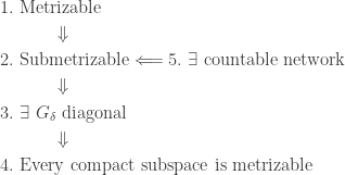
Let $(X, \tau)$ be a space. It is submetrizable if there is a topology $\tau_1$ on the set $X$ such that $\tau_1 \subset \tau$ and $(X, \tau_1)$ is a metrizable space. The topology $\tau_1$ is said to be weaker (coarser) than $\tau$ . Thus a space $X$ is submetrizable if it has a weaker metrizable topology.

Let $\mathcal{N}$ be a set of subsets of the space $X$ . $\mathcal{N}$ is said to be a network for $X$ if for every open subset $O$ of $X$ and for each $x \in O$ , there exists $N \in \mathcal{N}$ such that $x \in N \subset O$ . Having a network that is countable in size is a strong property (see here for a discussion on spaces with a countable network).

The diagonal of the space $X$ is the subset $\Delta=\left\{(x,x): x \in X \right\}$ of the square $X \times X$ . The space $X$ has a $G_\delta$ -diagonal if $\Delta$ is a $G_\delta$ -subset of $X \times X$ , i.e. $\Delta$ is the intersection of countably many open subsets of $X \times X$ .

The implication $1 \Longrightarrow 2$ is clear. For $5 \Longrightarrow 2$ , see Lemma 1 in this previous post on countable network. The implication $2 \Longrightarrow 3$ is left as an exercise. To see $3 \Longrightarrow 4$ , let $K$ be a compact subset of $X$ . The property of having a $G_\delta$ -diagonal is hereditary. Thus $K$ has a $G_\delta$ -diagonal. According to a well known result, any compact space with a $G_\delta$ -diagonal is metrizable (see here).

None of the implications in the diagram is reversible. The first uncountable ordinal $\omega_1$ is an example for $4 \not \Longrightarrow 3$ . This follows from the well known result that any countably compact space with a $G_\delta$ -diagonal is metrizable (see here). The Mrowka space is an example for $3 \not \Longrightarrow 2$ (see here). The Sorgenfrey line is an example for both $2 \not \Longrightarrow 5$ and $2 \not \Longrightarrow 1$ .

To see where the examples mentioned earlier are placed, note that Sorgenfrey line and Michael line are submetrizable, both are submetrizable by the usual Euclidean topology on the real line. Each compact subspace of the space $\omega_1$ is countable and is thus contained in some initial segment $[0,\alpha]$ which is metrizable. Any Moore space has a $G_\delta$ -diagonal. Thus compact subspaces of a Moore space are metrizable.

Function Spaces

We now look at some function spaces that are in the class “every compact subspace is metrizable.” For any Tychonoff space (completely regular space) $X$ , $C_p(X)$ is the space of all continuous functions from $X$ into $\mathbb{R}$ with the pointwise convergence topology (see here for basic information on pointwise convergence topology).

Theorem 1
Suppose that $X$ is a separable space. Then every compact subspace of $C_p(X)$ is metrizable.

Proof
The proof here actually shows more than is stated in the theorem. We show that $C_p(X)$ is submetrizable by a separable metric topology. Let $Y$ be a countable dense subspace of $X$ . Then $C_p(Y)$ is metrizable and separable since it is a subspace of the separable metric space $\mathbb{R}^{\omega}$ . Thus $C_p(Y)$ has a countable base. Let $\mathcal{E}$ be a countable base for $C_p(Y)$ .

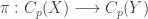
Let $\pi:C_p(X) \longrightarrow C_p(Y)$ be the restriction map, i.e. for each $f \in C_p(X)$ , $\pi(f)=f \upharpoonright Y$ . Since $\pi$ is a projection map, it is continuous and one-to-one and it maps $C_p(X)$ into $C_p(Y)$ . Thus $\pi$ is a continuous bijection from $C_p(X)$ into $C_p(Y)$ . Let $\mathcal{B}=\left\{\pi^{-1}(E): E \in \mathcal{E} \right\}$ .

We claim that $\mathcal{B}$ is a base for a topology on $C_p(X)$ . Once this is established, the proof of the theorem is completed. Note that $\mathcal{B}$ is countable and elements of $\mathcal{B}$ are open subsets of $C_p(X)$ . Thus the topology generated by $\mathcal{B}$ is coarser than the original topology of $C_p(X)$ .

For $\mathcal{B}$ to be a base, two conditions must be satisfied – $\mathcal{B}$ is a cover of $C_p(X)$ and for $B_1,B_2 \in \mathcal{B}$ , and for $f \in B_1 \cap B_2$ , there exists $B_3 \in \mathcal{B}$ such that $f \in B_3 \subset B_1 \cap B_2$ . Since $\mathcal{E}$ is a base for $C_p(Y)$ and since elements of $\mathcal{B}$ are preimages of elements of $\mathcal{E}$ under the map $\pi$ , it is straightforward to verify these two points. $\square$

Theorem 1 is actually a special case of a duality result in $C_p$ function space theory. More about this point later. First, consider a corollary of Theorem 1.

Corollary 2
Let $X=\prod_{\alpha<c} X_\alpha$ where $c$ is the cardinality continuum and each $X_\alpha$ is a separable space. Then every compact subspace of $C_p(X)$ is metrizable.

The key fact for Corollary 2 is that the product of continuum many separable spaces is separable (this fact is discussed here). Theorem 1 is actually a special case of a deep result.

Theorem 3
Suppose that $X=\prod_{\alpha<\kappa} X_\alpha$ is a product of separable spaces where $\kappa$ is any infinite cardinal. Then every compact subspace of $C_p(X)$ is metrizable.

Theorem 3 is a much more general result. The product of any arbitrary number of separable spaces is not separable if the number of factors is greater than continuum. So the proof for Theorem 1 will not work in the general case. This result is Problem 307 in [2].

A Duality Result

Theorem 1 is stated in a way that gives the right information for the purpose at hand. A more correct statement of Theorem 1 is: $X$ is separable if and only if $C_p(X)$ is submetrizable by a separable metric topology. Of course, the result in the literature is based on density and weak weight.

The cardinal function of density is the least cardinality of a dense subspace. For any space $Y$ , the weight of $Y$ , denoted by $w(Y)$ , is the least cardinaility of a base of $Y$ . The weak weight of a space $X$ is the least $w(Y)$ over all space $Y$ for which there is a continuous bijection from $X$ onto $Y$ . Thus if the weak weight of $X$ is $\omega$ , then there is a continuous bijection from $X$ onto some separable metric space, hence $X$ has a weaker separable metric topology.

There is a duality result between density and weak weight for $X$ and $C_p(X)$ . The duality result:

The density of $X$ coincides with the weak weight of $C_p(X)$ and the weak weight of $X$ coincides with the density of $C_p(X)$ . These are elementary results in $C_p$ -theory. See Theorem I.1.4 and Theorem I.1.5 in [1].

$\text{ }$

Reference

Arkhangelskii, A. V., Topological Function Spaces, Mathematics and Its Applications Series, Kluwer Academic Publishers, Dordrecht, 1992.
Tkachuk V. V., A $C_p$ -Theory Problem Book, Topological and Function Spaces, Springer, New York, 2011.

$\text{ }$

$\copyright$ 2017 – Dan Ma

The product of a perfectly normal space and a metric space is perfectly normal

Posted on March 1, 2017 by Dan Ma

The previous post gives a positive result for normality in product space. It shows that the product of a normal countably compact space and a metric space is always normal. In this post, we discuss another positive result, which is the following theorem.

Main Theorem
If $X$ is a perfectly normal space and $Y$ is a metric space, then $X \times Y$ is a perfectly normal space.

As a result of this theorem, perfectly normal spaces belong to a special class of spaces called P-spaces. K. Morita defined the notion of P-space and he proved that a space $Y$ is a Normal P-space if and only if $X \times Y$ is normal for every metric space $X$ (see the section below on P-spaces). Thus any perfectly normal space is a Normal P-space.

All spaces under consideration are Hausdorff. A subset $A$ of the space $X$ is a $G_\delta$ -subset of the space $X$ if $A$ is the intersection of countably many open subsets of $X$ . A subset $B$ of the space $X$ is an $F_\sigma$ -subset of the space $X$ if $B$ is the union of countably many closed subsets of $X$ . Clearly, a set $A$ is a $G_\delta$ -subset of the space $X$ if and only if $X-A$ is an $F_\sigma$ -subset of the space $X$ .

A space $X$ is said to be a perfectly normal space if $X$ is normal with the additional property that every closed subset of $X$ is a $G_\delta$ -subset of $X$ (or equivalently every open subset of $X$ is an $F_\sigma$ -subset of $X$ ).

The perfect normality has a characterization in terms of zero-sets and cozero-sets. A subset $A$ of the space $X$ is said to be a zero-set if there exists a continuous function $f: X \rightarrow [0,1]$ such that $A=f^{-1}(0)$ , where $f^{-1}(0)=\left\{x \in X: f(x)=0 \right\}$ . A subset $B$ of the space $X$ is a cozero-set if $X-B$ is a zero-set, or more explicitly if there is a continuous function $f: X \rightarrow [0,1]$ such that $B=\left\{x \in X: f(x)>0 \right\}$ .

It is well known that the space $X$ is perfectly normal if and only if every closed subset of $X$ is a zero-set, equivalently every open subset of $X$ is a cozero-set. See here for a proof of this result. We use this result to show that $X \times Y$ is perfectly normal.

____________________________________________________________________

The Proof

Let $X$ be a perfectly normal space and $Y$ be a metric space. Since $Y$ is a metric space, let $\mathcal{B}=\bigcup_{j=1}^\infty \mathcal{B}_j$ be a base for $Y$ such that each $\mathcal{B}_j$ is locally finite. We show that $X \times Y$ is perfectly normal. To that end, we show that every open subset of $X \times Y$ is a cozero-set. Let $U$ be an open subset of $X \times Y$ .

For each $(x,y) \in X \times Y$ , there exists open $O_{x,y} \subset X$ and there exists $B_{x,y} \in \mathcal{B}$ such that $(x,y) \in O_{x,y} \times B_{x,y} \subset U$ . Then $U$ is the union of all sets $O_{x,y} \times B_{x,y}$ . Observe that $B_{x,y} \in \mathcal{B}_{j}$ for some integer $j$ . For each $B \in \mathcal{B}$ such that $B=B_{x,y}$ for some $(x,y) \in X \times Y$ , let $O(B)$ be the union of all corresponding open sets $O_{x,y}$ for all applicable $(x,y)$ .

For each positive integer $j$ , let $\mathcal{W}_j$ be the collection of all open sets $O(B) \times B$ such that $B \in \mathcal{B}_j$ and $B=B_{x,y}$ for some $(x,y) \in X \times Y$ . Let $\mathcal{V}_j=\cup \mathcal{W}_j$ . As a result, $U=\bigcup_{j=1}^\infty \mathcal{V}_j$ .

Since both $X$ and $Y$ are perfectly normal, for each $O(B) \times B \in \mathcal{W}_j$ , there exist continuous functions

$F_{O(B),j}: X \rightarrow [0,1]$

$G_{B,j}: Y \rightarrow [0,1]$

such that

$O(B)=\left\{x \in X: F_{O(B),j}(x) >0 \right\}$

$B=\left\{y \in Y: G_{B,j}(y) >0 \right\}$

Now define $H_j: X \times Y \rightarrow [0,1]$ by the following:

$\displaystyle H_j(x,y)=\sum \limits_{O(B) \times B \in \mathcal{W}_j} F_{O(B),j}(x) \ G_{B,j}(y)$

for all $(x,y) \in X \times Y$ . Note that the function $H_j$ is well defined. Since $\mathcal{B}_j$ is locally finite in $Y$ , $\mathcal{W}_j$ is locally finite in $X \times Y$ . Thus $H_j(x,y)$ is obtained by summing a finite number of values of $F_{O(B),j}(x) \ G_{B,j}(y)$ . On the other hand, it can be shown that $H_j$ is continuous for each $j$ . Based on the definition of $H_j$ , it can be readily verified that $H_j(x,y)>0$ for all $(x,y) \in \cup \mathcal{W}_j$ and $H_j(x,y)=0$ for all $(x,y) \notin \cup \mathcal{W}_j$ .

Define $H: X \times Y \rightarrow [0,1]$ by the following:

$\displaystyle H(x,y)=\sum \limits_{j=1}^\infty \biggl[ \frac{1}{2^j} \ \frac{H_j(x,y)}{1+H_j(x,y)} \biggr]$

It is clear that $H$ is continuous. We claim that $U=\left\{(x,y) \in X \times Y: H(x,y) >0 \right\}$ . Recall that the open set $U$ is the union of all $O(B) \times B \in \mathcal{W}_j$ for all $j$ . Thus if $(x,y) \in \cup \mathcal{W}_j$ for some $j$ , then $H(x,y)>0$ since $H_j(x,y)>0$ . If $(x,y) \notin \cup \mathcal{W}_j$ for all $j$ , $H(x,y)=0$ since $H_j(x,y)=0$ for all $j$ . Thus the open set $U$ is an $F_\sigma$ -subset of $X \times Y$ . This concludes the proof that $X \times Y$ is perfectly normal. $\square$

____________________________________________________________________

Remarks

The main theorem here is a classic result in general topology. An alternative proof is to show that any perfectly normal space is a P-space (definition given below). Then by Morita’s theorem, the product of any perfectly normal space and any metric space is normal (Theorem 1 below). For another proof that is elementary, see Lemma 7 in this previous post.

The notions of perfectly normal spaces and paracompact spaces are quite different. By the theorem discussed here, perfectly normal spaces are normally productive with metric spaces. It is possible for a paracompact space to have a non-normal product with a metric space. The classic example is the Michael line (discussed here).

On the other hand, there are perfectly normal spaces that are not paracompact. One example is Bing’s Example H, which is perfectly normal and not paracompact (see here).

Even though a perfectly normal space is normally productive with metric spaces, it cannot be normally productive in general. For each non-discrete perfectly normal space $X$ , there exists a normal space $Y$ such that $X \times Y$ is not normal. This follows from Morita’s first conjecture (now a true statement). Morita’s first conjecture is discussed here.

____________________________________________________________________

P-Space in the Sense of Morita

Morita defined the notion of P-spaces [1] and [2]. Let $\kappa$ be a cardinal number such that $\kappa \ge 1$ . Let $\Gamma$ be the set of all finite ordered sequences $(\alpha_1,\alpha_2,\cdots,\alpha_n)$ where $n=1,2,\cdots$ and all $\alpha_i < \kappa$ . Let $X$ be a space. The collection $\left\{F_\sigma \subset X: \sigma \in \Gamma \right\}$ is said to be decreasing if this condition holds: $\sigma =(\alpha_1,\alpha_2,\cdots,\alpha_n)$ and $\delta =(\alpha_1,\alpha_2,\cdots,\alpha_n, \cdots, \alpha_m)$ with $n<m$ imply that $F_{\delta} \subset F_{\sigma}$ . The space $X$ is a P-space if for any cardinal $\kappa \ge 1$ and for any decreasing collection $\left\{F_\sigma \subset X: \sigma \in \Gamma \right\}$ of closed subsets of $X$ , there exists open set $U_\sigma$ for each $\sigma \in \Gamma$ such that the following conditions hold:

for all $\sigma \in \Gamma$ , $F_\sigma \subset U_\sigma$ ,
for any infinite sequence $(\alpha_1,\alpha_2,\cdots,\alpha_n,\cdots)$ where each each finite subsequence $\sigma_n=(\alpha_1,\alpha_2,\cdots,\alpha_n)$ is an element of $\Gamma$ , if $\bigcap_{n=1}^\infty F_{\sigma_n}=\varnothing$ , then $\bigcap_{n=1}^\infty U_{\sigma_n}=\varnothing$ .

If $\kappa=1$ where $1=\left\{0 \right\}$ . Then the index set $\Gamma$ defined above can be viewed as the set of all positive integers. As a result, the definition of P-space with $\kappa=1$ implies the a condition in Dowker’s theorem (see condition 6 in Theorem 1 here). Thus any space $X$ that is normal and a P-space is countably paracompact (or countably shrinking or that $X \times Y$ is normal for every compact metric space or any other equivalent condition in Dowker’s theorem). The following is a theorem of Morita.

Theorem 1 (Morita)
Let $X$ be a space. Then $X$ is a normal P-space if and only if $X \times Y$ is normal for every metric space $Y$ .

In light of Theorem 1, both perfectly normal spaces and normal countably compact spaces are P-spaces (see here). According to Theorem 1 and Dowker’s theorem, it follows that any normal P-space is countably paracompact.

____________________________________________________________________

Reference

Morita K., On the Product of a Normal Space with a Metric Space, Proc. Japan Acad., Vol. 39, 148-150, 1963. (article information; paper)
Morita K., Products of Normal Spaces with Metric Spaces, Math. Ann., Vol. 154, 365-382, 1964.

____________________________________________________________________
$\copyright \ 2017 \text{ by Dan Ma}$

The product of a normal countably compact space and a metric space is normal

Posted on February 5, 2017 by Dan Ma

It is well known that normality is not preserved by taking products. When nothing is known about the spaces $X$ and $Y$ other than the facts that they are normal spaces, there is not enough to go on for determining whether $X \times Y$ is normal. In fact even when one factor is a metric space and the other factor is a hereditarily paracompact space, the product can be non-normal (discussed here). This post discusses a productive scenario – the first factor is a normal space and second factor is a metric space with the first factor having the additional property that it is countably compact. In this scenario the product is always normal. This is a well known result in general topology. The goal here is to nail down a proof for use as future reference.

Main Theorem
Let $X$ be a normal and countably compact space. Then $X \times Y$ is a normal space for every metric space $Y$ .

The proof of the main theorem uses the notion of shrinkable open covers.

Remarks
The main theorem is a classic result and is often used as motivation for more advanced results for products of normal spaces. Thus we would like to present a clear and complete proof of this classic result for anyone who would like to study the topics of normality (or the lack of) in product spaces. We found that some proofs of this result in the literature are hard to follow. In A. H. Stone’s paper [2], the result is stated in a footnote, stating that “it can be shown that the topological product of a metric space and a normal countably compact space is normal, though not necessarily paracompact”. We had seen several other papers citing [2] as a reference for the result. The Handbook [1] also has a proof (Corollary 4.10 in page 805), which we feel may not be the best proof to learn from. We found a good proof in [3] using the idea of shrinking of open covers.

____________________________________________________________________

The Notion of Shrinking

The key to the proof is the notion of shrinkable open covers and shrinking spaces. Let $X$ be a space. Let $\mathcal{U}$ be an open cover of $X$ . The open cover of $\mathcal{U}$ is said to be shrinkable if there is an open cover $\mathcal{V}=\left\{V(U): U \in \mathcal{U} \right\}$ of $X$ such that $\overline{V(U)} \subset U$ for each $U \in \mathcal{U}$ . When this is the case, the open cover $\mathcal{V}$ is said to be a shrinking of $\mathcal{U}$ . If an open cover is shrinkable, we also say that the open cover can be shrunk (or has a shrinking). Whenever an open cover has a shrinking, the shrinking is indexed by the open cover that is being shrunk. Thus if the original cover is indexed, e.g. $\left\{U_\alpha: \alpha<\kappa \right\}$ , then a shrinking has the same indexing, e.g. $\left\{V_\alpha: \alpha<\kappa \right\}$ .

A space $X$ is a shrinking space if every open cover of $X$ is shrinkable. Every open cover of a paracompact space has a locally finite open refinement. With a little bit of rearranging, the locally finite open refinement can be made to be a shrinking (see Theorem 2 here). Thus every paracompact space is a shrinking space. For other spaces, the shrinking phenomenon is limited to certain types of open covers. In a normal space, every finite open cover has a shrinking, as stated in the following theorem.

Theorem 1
The following conditions are equivalent.

The space $X$ is normal.
Every point-finite open cover of $X$ is shrinkable.
Every locally finite open cover of $X$ is shrinkable.
Every finite open cover of $X$ is shrinkable.
Every two-element open cover of $X$ is shrinkable.

The hardest direction in the proof is $1 \Longrightarrow 2$ , which is established in this previous post. The directions $2 \Longrightarrow 3 \Longrightarrow 4 \Longrightarrow 5$ are immediate. To see $5 \Longrightarrow 1$ , let $H$ and $K$ be two disjoint closed subsets of $X$ . By condition 5, the two-element open cover $\left\{X-H,X-K \right\}$ has a shrinking $\left\{U,V \right\}$ . Then $\overline{U} \subset X-H$ and $\overline{V} \subset X-K$ . As a result, $H \subset X-\overline{U}$ and $K \subset X-\overline{V}$ . Since the open sets $U$ and $V$ cover the whole space, $X-\overline{U}$ and $X-\overline{V}$ are disjoint open sets. Thus $X$ is normal.

In a normal space, all finite open covers are shrinkable. In general, an infinite open cover of a normal space may or may not be shrinkable. It turns out that finding a normal space with an infinite open cover that is not shrinkable is no trivial matter (see Dowker’s theorem in this previous post). However, if an open cover in a normal space is point-finite or locally finite, then it is shrinkable.

____________________________________________________________________

Key Idea

We now discuss the key idea to the proof of the main theorem. Consider the product space $X \times Y$ . Let $\mathcal{U}$ be an open cover of $X \times Y$ . Let $M \subset Y$ . The set $M$ is stable with respect to the open cover $\mathcal{U}$ if for each $x \in X$ , there is an open set $O_x$ containing $x$ such that $O_x \times M \subset U$ for some $U \in \mathcal{U}$ .

Let $\kappa$ be a cardinal number (either finite or infinite). A space $X$ is a $\kappa$ -shrinking space if for each open cover $\mathcal{W}$ of $X$ such that the cardinality of $\mathcal{W}$ is $\le \kappa$ , then $\mathcal{W}$ is shrinkable. According to Theorem 1, any normal space is 2-shrinkable.

Theorem 2
Let $\kappa$ be a cardinal number (either finite or infinite). Let $X$ be a $\kappa$ -shrinking space. Let $Y$ be a paracompact space. Suppose that $\mathcal{U}$ is an open cover of $X \times Y$ such that the following two conditions are satisfied:

Each point $y \in Y$ has an open set $V_y$ containing $y$ such that $V_y$ is stable with respect to $\mathcal{U}$ .
$\lvert \mathcal{U} \lvert = \kappa$ .

Then $\mathcal{U}$ is shrinkable.

Proof of Theorem 2
Let $\mathcal{U}$ be any open cover of $X \times Y$ satisfying the hypothesis. We show that $\mathcal{U}$ has a shrinking.

For each $y \in Y$ , obtain the open covers $\left\{G(U,y): U \in \mathcal{U} \right\}$ and $\left\{H(U,y): U \in \mathcal{U} \right\}$ of $X$ as follows. For each $U \in \mathcal{U}$ , define the following:

$G(U,y)=\cup \left\{O: O \text{ is open in } X \text{ such that } O \times V_y \subset U \right\}$

Then $\left\{G(U,y): U \in \mathcal{U} \right\}$ is an open cover of $X$ . Since $X$ is $\kappa$ -shrinkable, there is an open cover $\left\{H(U,y): U \in \mathcal{U} \right\}$ of $X$ such that $\overline{H(U,y)} \subset G(U,y)$ for each $U \in \mathcal{U}$ .

Now $\left\{V_y: y \in Y \right\}$ is an open cover of $Y$ . By the paracompactness of $Y$ , let $\left\{W_y: y \in Y \right\}$ be a locally finite open cover of $Y$ such that $\overline{W_y} \subset V_y$ for each $y \in Y$ . For each $U \in \mathcal{U}$ , define the following:

$W_U=\cup \left\{H(U,y) \times W_y: y \in Y \text{ such that } \overline{H(U,y) \times W_y} \subset U \right\}$

We claim that $\mathcal{W}=\left\{ W_U: U \in \mathcal{U} \right\}$ is a shrinking of $\mathcal{U}$ . First it is a cover of $X \times Y$ . Let $(x,t) \in X \times Y$ . Then $t \in W_y$ for some $y \in Y$ . There exists $U \in \mathcal{U}$ such that $x \in H(U,y)$ . Note the following.

$\overline{H(U,y) \times W_y} \subset \overline{H(U,y)} \times \overline{W_y} \subset G(U,y) \times V_y \subset U$

This means that $H(U,y) \times W_y \subset W_U$ . Since $(x,t) \in H(U,y) \times W_y$ , $(x,t) \in W_U$ . Thus $\mathcal{W}$ is an open cover of $X \times Y$ .

Now we show that $\mathcal{W}$ is a shrinking of $\mathcal{U}$ . Let $U \in \mathcal{U}$ . To show that $\overline{W_U} \subset U$ , let $(x,t) \in \overline{W_U}$ . Let $L$ be open in $Y$ such that $t \in L$ and that $L$ meets only finitely many $W_y$ , say for $y=y_1,y_2,\cdots,y_n$ . Immediately we have the following relations.

$\forall \ i=1,\cdots,n, \ \overline{W_{y_i}} \subset V_{y_i}$

$\forall \ i=1,\cdots,n, \ \overline{H(U,y_i)} \subset G(U,y_i)$

$\forall \ i=1,\cdots,n, \ \overline{H(U,y_i) \times W_{y_i}} \subset \overline{H(U,y_i)} \times \overline{W_{y_i}} \subset G(U,y_i) \times V_{y_i} \subset U$

Then it follows that

$\displaystyle (x,t) \in \overline{\bigcup \limits_{j=1}^n H(U,y_j) \times W_{y_j}}=\bigcup \limits_{j=1}^n \overline{H(U,y_j) \times W_{y_j}} \subset U$

Thus $U \in \mathcal{U}$ . This shows that $\mathcal{W}$ is a shrinking of $\mathcal{U}$ . $\square$

Remark
Theorem 2 is the Theorem 3.2 in [3]. Theorem 2 is a formulation of Theorem 3.2 [3] for the purpose of proving Theorem 3 below.

____________________________________________________________________

Main Theorem

Theorem 3 (Main Theorem)
Let $X$ be a normal and countably compact space. Let $Y$ be a metric space. Then $X \times Y$ is a normal space.

Proof of Theorem 3
Let $\mathcal{U}$ be a 2-element open cover of $X \times Y$ . We show that $\mathcal{U}$ is shrinkable. This would mean that $X \times Y$ is normal (according to Theorem 1). To show that $\mathcal{U}$ is shrinkable, we show that the open cover $\mathcal{U}$ satisfies the two bullet points in Theorem 2.

Fix $y \in Y$ . Let $\left\{B_n: n=1,2,3,\cdots \right\}$ be a base at the point $y$ . Define $G_n$ as follows:

$G_n=\cup \left\{O \subset X: O \text{ is open such that } O \times B_n \subset U \text{ for some } U \in \mathcal{U} \right\}$

It is clear that $\mathcal{G}=\left\{G_n: n=1,2,3,\cdots \right\}$ is an open cover of $X$ . Since $X$ is countably compact, choose $m$ such that $\left\{G_1,G_2,\cdots,G_m \right\}$ is a cover of $X$ . Let $E_y=\bigcap_{j=1}^m B_j$ . We claim that $E_y$ is stable with respect to $\mathcal{U}$ . To see this, let $x \in X$ . Then $x \in G_j$ for some $j \le m$ . By the definition of $G_j$ , there is some open set $O_x \subset X$ such that $x \in O_x$ and $O_x \times B_j \subset U$ for some $U \in \mathcal{U}$ . Furthermore, $O_x \times E_y \subset O_x \times B_j \subset U$ .

To summarize: for each $y \in Y$ , there is an open set $E_y$ such that $y \in E_y$ and $E_y$ is stable with respect to the open cover $\mathcal{U}$ . Thus the first bullet point of Theorem 2 is satisfied. The open cover $\mathcal{U}$ is a 2-element open cover. Thus the second bullet point of Theorem 2 is satisfied. By Theorem 2, the open cover $\mathcal{U}$ is shrinkable. Thus $X \times Y$ is normal. $\square$

Corollary 4
Let $X$ be a normal and pseudocompact space. Let $Y$ be a metric space. Then $X \times Y$ is a normal space.

The corollary follows from the fact that any normal and pseudocompact space is countably compact (see here).

Remarks
The proof of Theorem 3 actually gives a more general result. Note that the second factor only needs to be paracompact and that every point has a countable base (i.e. first countable). The first factor $X$ has to be countably compact. The shrinking requirement for $X$ is flexible – if open covers of a certain size for $X$ are shrinkable, then open covers of that size for the product are shrinkable. We have the following corollaries.

Corollary 5
Let $X$ be a $\kappa$ -shrinking and countably compact space and let $Y$ be a paracompact first countable space. Then $X \times Y$ is a $\kappa$ -shrinking space.

Corollary 6
Let $X$ be a shrinking and countably compact space and let $Y$ be a paracompact first countable space. Then $X \times Y$ is a shrinking space.

____________________________________________________________________

Remarks

The main theorem (Theorem 3) says that any normal and countably compact space is productively normal with one class of spaces, namely the metric spaces. Thus if one wishes to find a non-normal product space with one factor being countably compact, the other factor must not be a metric space. For example, if $W=\omega_1$ , the first uncountable ordinal with the ordered topology, then $W \times X$ is always normal for every metric $X$ . For non-normal example, $W \times C$ is not normal for any compact space $C$ with uncountable tightness (see Theorem 1 in this previous post). Another example, $W \times L_{\omega_1}$ is not normal where $L_{\omega_1}$ is the one-point Lindelofication of a discrete space of cardinality $\omega_1$ (follows from Example 1 and Theorem 7 in this previous post).

Another comment is that normal countably paracompact spaces are examples of Normal P-spaces. K. Morita defined the notion of P-space and he proved that a space $Y$ is a Normal P-space if and only if $X \times Y$ is normal for every metric space $X$ .

____________________________________________________________________

Reference

Przymusinski T. C., Products of Normal Spaces, Handbook of Set-Theoretic Topology (K. Kunen and J. E. Vaughan, eds), Elsevier Science Publishers B. V., Amsterdam, 781-826, 1984.
Stone A. H., Paracompactness and Product Spaces, Bull. Amer. Math. Soc., Vol. 54, 977-982, 1948. (paper)
Yang L., The Normality in Products with a Countably Compact Factor, Canad. Math. Bull., Vol. 41 (2), 245-251, 1998. (abstract, paper)

____________________________________________________________________
$\copyright \ 2017 \text{ by Dan Ma}$

The product of uncountably many factors is never hereditarily normal

Posted on May 3, 2015 by Dan Ma

The space $Y=\prod_{\alpha<\omega_1} \left\{0,1 \right\}=\left\{0,1 \right\}^{\omega_1}$ is the product of $\omega_1$ many copies of the two-element set $\left\{0,1 \right\}$ where $\omega_1$ is the first uncountable ordinal. It is a compact space by Tychonoff’s theorem. It is a normal space since every compact Hausdorff space is normal. A space is hereditarily normal if every subspace is normal. Is the space $Y$ hereditarily normal? In this post, we give two proofs that it is not hereditarily normal. It then follows that any product space $\prod X_\alpha$ cannot be hereditarily normal as long as there are uncountably many factors and every factor has at least two point.

____________________________________________________________________

The connection with a theorem of Katetov

It turns out that there is a connection with a theorem of Katetov. For any compact space, knowing hereditary normality of the first several self product spaces can reveal a great deal of information about the compact space. More specifically, for any compact space $X$ , knowing whether $X$ , $X^2$ and $X^3$ are hereditarily normal can tell us whether $X$ is metrizable. If all three are hereditarily normal, then $X$ is metrizable. If one of the three self products is not hereditarily normal, then $X$ is not metrizable. This fact is based on a theorem of Katetov (see this previous post). The space $Y=\left\{0,1 \right\}^{\omega_1}$ is not metrizable since it is not first countable (see Problem 1 below). Thus one of its first three self products must fail to be hereditarily normal.

These two proofs are not direct proof in the sense that a non-normal subspace is not explicitly produced. Instead the proofs use other theorem or basic but important background results. One of the two proofs (#2) uses a theorem of Katetov on hereditarily normal spaces. The other proof (#1) uses the fact that the product of uncountably many copies of a countable discrete space is not normal. We believe that these two proofs and the required basic facts are an important training ground for topology. We list out these basic facts as exercises. Anyone who wishes to fill in the gaps can do so either by studying the links provided or by consulting other sources.

The theorem of Katetov mentioned earlier provides a great exercise – for any non-metrizable compact space $X$ , determine where the hereditary normality fails. Does it fail in $X$ , $X^2$ or $X^3$ ? This previous post examines a small list of compact non-metrizable spaces. In all the examples in this list, the hereditary normality fails in $X$ or $X^2$ . The space $Y=\left\{0,1 \right\}^{\omega_1}$ can be added to this list. All the examples in this list are defined using no additional set theory axioms beyond ZFC. A natural question: does there exist an example of compact non-metrizable space $X$ such that the hereditary normality holds in $X^2$ and fails in $X^3$ ? It turns out that this was a hard problem and the answer is independent of ZFC. This previous post provides a brief discussion and has references for the problem.

All spaces under consideration are Hausdorff spaces.

____________________________________________________________________

Exercises

Problem 1
Let $X$ be a compact space. Show that $X$ is normal.

Problem 2
For each $\alpha<\omega_1$ , let $A_\alpha$ be a set with cardinality $\le \omega_1$ . Show that $\lvert \bigcup_{\alpha<\omega_1} A_\alpha \lvert \le \omega_1$ .

Problem 2 holds for any infinite cardinal, not just $\omega_1$ . One reference for Problem 2 is Lemma 10.21 on page 30 of Set Theorey, An Introduction to Independence Proofs by Kenneth Kunen.

Problem 3
For each $\alpha<\omega_1$ , let $X_\alpha$ be a space with at least two points. Show that for every point $p \in \prod_{\alpha<\omega_1} X_\alpha$ , there does not exist a countable base at the point $p$ . In other words, the product space $\prod_{\alpha<\omega_1} X_\alpha$ is not first countable at every point. It follows that product space $\prod_{\alpha<\omega_1} X_\alpha$ is not metrizable.

Problem 4
In any space, a $G_\delta$ -set is a set that is the intersection of countably many open sets. When a singleton set $\left\{ x \right\}$ is a $G_\delta$ -set, we say the point $x$ is a $G_\delta$ -point. For each $\alpha<\omega_1$ , let $X_\alpha$ be a space with at least two points. Show that every point $p$ in the product space $\prod_{\alpha<\omega_1} X_\alpha$ is not a $G_\delta$ -point.

Note that Problem 4 implies Problem 3.

For Problem 3 and Problem 4, use the fact that there are uncountably many factors and that a basic open set in the product space is of the form $\prod_{\alpha<\omega_1} O_\alpha$ and that it has only finitely many coordinates at which $O_\alpha \ne X_\alpha$ .

Problem 5
For each $\alpha<\omega_1$ , let $X_\alpha=\left\{0,1,2,\cdots \right\}$ be the set of non-negative integers with the discrete topology. Show that the product space $\prod_{\alpha<\omega_1} X_\alpha$ is not normal.

See here for a discussion of Problem 5.

Problem 6
Let $\displaystyle Y=\left\{0,1 \right\}^{\omega_1}$ . Show that $Y$ has a countably infinite subspace

$W=\left\{y_0,y_1,y_2,y_3\cdots \right\}$

such that $W$ is relatively discrete. In other words, $W$ is discrete in the subspace topology of $W$ . However $W$ is not discrete in the product space $Y$ since $Y$ is compact.

____________________________________________________________________

Proof #1

Let $\displaystyle Y=\left\{0,1 \right\}^{\omega_1}$ . We show that $Y$ is not hereditarily normal.

Note that the product space $\displaystyle Y=\left\{0,1 \right\}^{\omega_1}$ can be written as the product of $\omega_1$ many copies of itself:

$\displaystyle \left\{0,1 \right\}^{\omega_1} \cong \left\{0,1 \right\}^{\omega_1} \times \left\{0,1 \right\}^{\omega_1} \times \left\{0,1 \right\}^{\omega_1} \times \cdots \ \ \ \ \ \ \ \ \ \ \ \ \ \ \ \ \ \ \ \ \ (1)$

The fact (1) follows from the fact that the union of $\omega_1$ many pairwise disjoint sets, each of which has cardinality $\omega_1$ , has cardinality $\omega_1$ (see Problem 2). The space $\left\{0,1 \right\}^{\omega_1}$ has a countably infinite subspace that is relatively discrete (see Problem 6). In other words, it has a subspace that is homemorphic to $\omega=\left\{0,1,2,\cdots \right\}$ where $\omega$ has the discrete topology. Thus the following is homeomorphic to a subspace of $\displaystyle Y=\left\{0,1 \right\}^{\omega_1}$ .

$\displaystyle \omega^{\omega_1} = \omega \times \omega \times \omega \times \cdots \ \ \ \ \ \ \ \ \ \ \ \ \ \ \ \ \ \ \ \ \ \ \ \ \ \ \ \ \ \ \ \ \ \ \ \ \ \ \ \ \ \ \ \ \ \ \ \ \ \ \ (2)$

By Problem 5, the space $\omega^{\omega_1}$ is not normal. Hence the compact space $\displaystyle Y=\left\{0,1 \right\}^{\omega_1}$ contains the non-normal space $\omega^{\omega_1}$ and is thus not hereditarily normal. $\blacksquare$

____________________________________________________________________

Proof #2

Let $\displaystyle Y=\left\{0,1 \right\}^{\omega_1}$ . We show that $Y$ is not hereditarily normal. This proof uses a theorem of Katetov, discussed in this previous post and stated below.

Theorem 1
If $X_1 \times X_2$ is hereditarily normal (i.e. every one of its subspaces is normal), then one of the following condition holds:

The factor $X_1$ is perfectly normal.
Every countable and infinite subset of the factor $X_2$ is closed.

First, $Y$ can be written as the product of two copies of itself:

$\displaystyle \left\{0,1 \right\}^{\omega_1} \cong \left\{0,1 \right\}^{\omega_1} \times \left\{0,1 \right\}^{\omega_1} \ \ \ \ \ \ \ \ \ \ \ \ \ \ \ \ \ \ \ \ \ \ \ \ \ \ \ \ \ \ \ \ \ \ \ \ \ \ \ \ \ \ \ (3)$

This is because the union of two disjoints sets, each of which has cardinality $\omega_1$ , has carinality $\omega_1$ . Note that the countably infinite subset $W$ from Problem 6 is not a closed subset of $Y$ . If it were, the compact space $Y$ would contain an infinite set with no limit point. Thus the second condition of Theorem 1 is not satisfied. If $Y \cong Y \times Y$ were to be hereditarily normal, then the first condition must be satisfied, i.e. $Y$ is perfectly normal (meaning that $Y$ is normal and that every closed subset of it is a $G_\delta$ -set). However, Problem 4 indicates that no point in $Y$ can be a $G_\delta$ point. Therefore $Y$ cannot be hereditarily normal. $\blacksquare$

____________________________________________________________________

Corollary

The product of uncountably many spaces, each one of which has at least two points, contains a homeomorphic copy of the space $\displaystyle Y=\left\{0,1 \right\}^{\omega_1}$ . Thus such a product space can never be hereditarily normal. We state this more formally below.

Theorem 2
Let $\kappa$ be any uncountable cardinal. For each $\alpha<\kappa$ , let $X_\alpha$ be a space with at least two points. Then $\prod_{\alpha<\kappa} X_\alpha$ is not hereditarily normal.

____________________________________________________________________
$\copyright \ 2015 \text{ by Dan Ma}$

Compact metrizable scattered spaces

Posted on April 1, 2015 by Dan Ma

A scattered space is one in which there are isolated points found in every subspace. Specifically, a space $X$ is a scattered space if every non-empty subspace $Y$ of $X$ has a point $y \in Y$ such that $y$ is an isolated point in $Y$ , i.e. the singleton set $\left\{y \right\}$ is open in the subspace $Y$ . A handy example is a space consisting of ordinals. Note that in a space of ordinals, every non-empty subset has an isolated point (e.g. its least element). In this post, we discuss scattered spaces that are compact metrizable spaces.

Here’s what led the author to think of such spaces. Consider Theorem III.1.2 found on page 91 of Arhangelskii’s book on topological function space [1], which is Theorem 1 stated below:

Thereom 1
For any compact space $X$ , the following conditions are equivalent:

The function space $C_p(X)$ is a Frechet-Urysohn space.
The function space $C_p(X)$ is a k space.
$X$ is a scattered space.

Let’s put aside the Frechet-Urysohn property and the k space property for the moment. For any Hausdorff space $X$ , let $C(X)$ be the set of all continuous real-valued functions defined on the space $X$ . Since $C(X)$ is a subspace of the product space $\mathbb{R}^X$ , a natural topology that can be given to $C(X)$ is the subspace topology inherited from the product space $\mathbb{R}^X$ . Then $C_p(X)$ is simply the set $C(X)$ with the product subspace topology (also called the pointwise convergence topology).

Let’s say the compact space $X$ is countable and infinite. Then the function space $C_p(X)$ is metrizable since it is a subspace of $\mathbb{R}^X$ , a product of countably many lines. Thus the function space $C_p(X)$ has the Frechet-Urysohn property (being metrizable implies Frechet-Urysohn). This means that the compact space $X$ is scattered. The observation just made is a proof that any infinite compact space that is countable in cardinality must be scattered. In particular, every infinite compact and countable space must have an isolated point. There must be a more direct proof of this same fact without taking the route of a function space. The indirect argument does not reveal the essential nature of compact metric spaces. The essential fact is that any uncountable compact metrizable space contains a Cantor set, which is as unscattered as any space can be. Thus the only scattered compact metrizable spaces are the countable ones.

The main part of the proof is the construction of a Cantor set in a compact metrizable space (Theorem 3). The main result is Theorem 4. In many settings, the construction of a Cantor set is done in the real number line (e.g. the middle third Cantor set). The construction here is in a more general setting. But the idea is still the same binary division process – the splitting of a small open set with compact closure into two open sets with disjoint compact closure. We also use that fact that any compact metric space is hereditarily Lindelof (Theorem 2).

____________________________________________________________________

Compact metrizable spaces

We first define some notions before looking at compact metrizable spaces in more details. Let $X$ be a space. Let $A \subset X$ . Let $p \in X$ . We say that $p$ is a limit point of $A$ if every open subset of $X$ containing $p$ contains a point of $A$ distinct from $p$ . So the notion of limit point here is from a topology perspective and not from a metric perspective. In a topological space, a limit point does not necessarily mean that it is the limit of a convergent sequence (however, it does in a metric space). The proof of the following theorem is straightforward.

Theorem 2
Let $X$ be a hereditarily Lindelof space (i.e. every subspace of $X$ is Lindelof). Then for any uncountable subset $A$ of $X$ , all but countably many points of $A$ are limit points of $A$ .

We now discuss the main result.

Theorem 3
Let $X$ be a compact metrizable space such that every point of $X$ is a limit point of $X$ . Then there exists an uncountable closed subset $C$ of $X$ such that every point of $C$ is a limit point of $C$ .

Proof of Theorem 3
Note that any compact metrizable space is a complete metric space. Consider a complete metric $\rho$ on the space $X$ . One fact that we will use is that if there is a sequence of closed sets $X \supset H_1 \supset H_2 \supset H_3 \supset \cdots$ such that the diameters of the sets $H$ (based on the complete metric $\rho$ ) decrease to zero, then the sets $H_n$ collapse to one point.

The uncountable closed set $C$ we wish to define is a Cantor set, which is constructed from a binary division process. To start, pick two points $p_0,p_1 \in X$ such that $p_0 \ne p_1$ . By assumption, both points are limit points of the space $X$ . Choose open sets $U_0,U_1 \subset X$ such that

$p_0 \in U_0$ ,
$p_1 \in U_1$ ,
$K_0=\overline{U_0}$ and $K_1=\overline{U_1}$ ,
$K_0 \cap K_1 = \varnothing$ ,
the diameters for $K_0$ and $K_1$ with respect to $\rho$ are less than 0.5.

Note that each of these open sets contains infinitely many points of $X$ . Then we can pick two points in each of $U_0$ and $U_1$ in the same manner. Before continuing, we set some notation. If $\sigma$ is an ordered string of 0’s and 1’s of length $n$ (e.g. 01101 is a string of length 5), then we can always extend it by tagging on a 0 and a 1. Thus $\sigma$ is extended as $\sigma 0$ and $\sigma 1$ (e.g. 01101 is extended by 011010 and 011011).

Suppose that the construction at the $n$ th stage where $n \ge 1$ is completed. This means that the points $p_\sigma$ and the open sets $U_\sigma$ have been chosen such that $p_\sigma \in U_\sigma$ for each length $n$ string of 0’s and 1’s $\sigma$ . Now we continue the picking for the $(n+1)$ st stage. For each $\sigma$ , an $n$ -length string of 0’s and 1’s, choose two points $p_{\sigma 0}$ and $p_{\sigma 1}$ and choose two open sets $U_{\sigma 0}$ and $U_{\sigma 1}$ such that

$p_{\sigma 0} \in U_{\sigma 0}$ ,
$p_{\sigma 1} \in U_{\sigma 1}$ ,
$K_{\sigma 0}=\overline{U_{\sigma 0}} \subset U_{\sigma}$ and $K_{\sigma 1}=\overline{U_{\sigma 1}} \subset U_{\sigma}$ ,
$K_{\sigma 0} \cap K_{\sigma 1} = \varnothing$ ,
the diameters for $K_{\sigma 0}$ and $K_{\sigma 1}$ with respect to $\rho$ are less than $0.5^{n+1}$ .

For each positive integer $m$ , let $C_m$ be the union of all $K_\sigma$ over all $\sigma$ that are $m$ -length strings of 0’s and 1’s. Each $C_m$ is a union of finitely many compact sets and is thus compact. Furthermore, $C_1 \supset C_2 \supset C_3 \supset \cdots$ . Thus $C=\bigcap \limits_{m=1}^\infty C_m$ is non-empty. To complete the proof, we need to show that

$C$ is uncountable (in fact of cardinality continuum),
every point of $C$ is a limit point of $C$ .

To show the first point, we define a one-to-one function $f: \left\{0,1 \right\}^N \rightarrow C$ where $N=\left\{1,2,3,\cdots \right\}$ . Note that each element of $\left\{0,1 \right\}^N$ is a countably infinite string of 0’s and 1’s. For each $\tau \in \left\{0,1 \right\}^N$ , let $\tau \upharpoonright n$ denote the string of the first $n$ digits of $\tau$ . For each $\tau \in \left\{0,1 \right\}^N$ , let $f(\tau)$ be the unique point in the following intersection:

$\displaystyle \bigcap \limits_{n=1}^\infty K_{\tau \upharpoonright n} = \left\{f(\tau) \right\}$

This mapping is uniquely defined. Simply conceptually trace through the induction steps. For example, if $\tau$ are 01011010…., then consider $K_0 \supset K_{01} \supset K_{010} \supset \cdots$ . At each next step, always pick the $K_{\tau \upharpoonright n}$ that matches the next digit of $\tau$ . Since the sets $K_{\tau \upharpoonright n}$ are chosen to have diameters decreasing to zero, the intersection must have a unique element. This is because we are working in a complete metric space.

It is clear that the map $f$ is one-to-one. If $\tau$ and $\gamma$ are two different strings of 0’s and 1’s, then they must differ at some coordinate, then from the way the induction is done, the strings would lead to two different points. It is also clear to see that the map $f$ is reversible. Pick any point $x \in C$ . Then the point $x$ must belong to a nested sequence of sets $K$ ‘s. This maps to a unique infinite string of 0’s and 1’s. Thus the set $C$ has the same cardinality as the set $\left\{0,1 \right\}^N$ , which has cardinality continuum.

To see the second point, pick $x \in C$ . Suppose $x=f(\tau)$ where $\tau \in \left\{0,1 \right\}^N$ . Consider the open sets $U_{\tau \upharpoonright n}$ for all positive integers $n$ . Note that $x \in U_{\tau \upharpoonright n}$ for each $n$ . Based on the induction process described earlier, observe these two facts. This sequence of open sets has diameters decreasing to zero. Each open set $U_{\tau \upharpoonright n}$ contains infinitely many other points of $C$ (this is because of all the open sets $U_{\tau \upharpoonright k}$ that are subsets of $U_{\tau \upharpoonright n}$ where $k \ge n$ ). Because the diameters are decreasing to zero, the sequence of $U_{\tau \upharpoonright n}$ is a local base at the point $x$ . Thus, the point $x$ is a limit point of $C$ . This completes the proof. $\blacksquare$

Theorem 4
Let $X$ be a compact metrizable space. It follows that $X$ is scattered if and only if $X$ is countable.

Proof of Theorem 4
$\Longleftarrow$
In this direction, we show that if $X$ is countable, then $X$ is scattered (the fact that can be shown using the function space argument pointed out earlier). Here, we show the contrapositive: if $X$ is not scattered, then $X$ is uncountable. Suppose $X$ is not scattered. Then every point of $X$ is a limit point of $X$ . By Theorem 3, $X$ would contain a Cantor set $C$ of cardinality continuum.

$\Longrightarrow$
In this direction, we show that if $X$ is scattered, then $X$ is countable. We also show the contrapositive: if $X$ is uncountable, then $X$ is not scattered. Suppose $X$ is uncountable. By Theorem 2, all but countably many points of $X$ are limit points of $X$ . After discarding these countably many isolated points, we still have a compact space. So we can just assume that every point of $X$ is a limit point of $X$ . Then by Theorem 3, $X$ contains an uncountable closed set $C$ such that every point of $C$ is a limit point of $C$ . This means that $X$ is not scattered. $\blacksquare$

____________________________________________________________________

Remarks

A corollary to the above discussion is that the cardinality for any compact metrizable space is either countable (including finite) or continuum (the cardinality of the real line). There is nothing in between or higher than continuum. To see this, the cardinality of any Lindelof first countable space is at most continuum according to a theorem in this previous post (any compact metric space is one such). So continuum is an upper bound on the cardinality of compact metric spaces. Theorem 3 above implies that any uncountable compact metrizable space has to contain a Cantor set, hence has cardinality continuum. So the cardinality of a compact metrizable space can be one of two possibilities – countable or continuum. Even under the assumption of the negation of the continuum hypothesis, there will be no uncountable compact metric space of cardinality less than continuum. On the other hand, there is only one possibility for the cardinality of a scattered compact metrizable, which is countable.

____________________________________________________________________

Reference

Arkhangelskii, A. V., Topological Function Spaces, Mathematics and Its Applications Series, Kluwer Academic Publishers, Dordrecht, 1992.

____________________________________________________________________
$\copyright \ 2015 \text{ by Dan Ma}$

A useful lemma for proving normality

Posted on July 4, 2014 by Dan Ma

In this post we discuss a lemma (Lemma 1 below) that is useful for proving normality. In some cases, it is more natural using this lemma to prove that a space is normal than using the definition of normality. The proof of Lemma 1 is not difficult. Yet it simplifies some proofs of normality. One reason is that the derivation of two disjoint open sets that are to separate two disjoint closed sets is done in the lemma, thus simplifying the main proof at hand. The lemma is well known and is widely used in the literature. See Lemma 1.5.15 in [1]. Two advanced examples of applications are [2] and [3]. After proving the lemma, we give three elementary applications of the lemma. One of the applications is a characterization of perfectly normal spaces. This characterization is, in some cases, easier to use, e.g. making it easy to show that perfectly normal implies hereditarily normal.

In this post, we only consider spaces that are regular and $T_1$ . A space $X$ is regular if for each open set $U \subset X$ and for each $x \in U$ , there exists an open $V \subset X$ with $x \in V \subset \overline{V} \subset U$ . A space is $T_1$ if every set with only one point is a closed set.

Lemma 1
A space $Y$ is a normal space if the following condition (Condition 1) is satisfied:

For each closed subset $L$ of $Y$ , and for each open subset $M$ of $Y$ with $L \subset M$ , there exists a sequence $M_1,M_2,M_3,\cdots$ of open subsets of $Y$ such that $L \subset \bigcup_{i=1}^\infty M_i$ and $\overline{M_i} \subset M$ for each $i$ .

Proof of Lemma 1
Suppose the space $Y$ satisfies condition 1. Let $H$ and $K$ be disjoint closed subsets of the space $Y$ . Consider $H \subset U=Y \backslash K$ . Using condition 1, there exists a sequence $U_1,U_2,U_3,\cdots$ of open subsets of the space $Y$ such that $H \subset \bigcup_{i=1}^\infty U_i$ and $\overline{U_i} \cap K=\varnothing$ for each $i$ . Consider $K \subset V=Y \backslash H$ . Similarly, there exists a sequence $V_1,V_2,V_3,\cdots$ of open subsets of the space $Y$ such that $K \subset \bigcup_{i=1}^\infty V_i$ and $\overline{V_i} \cap H=\varnothing$ for each $i$ .

For each positive integer $n$ , define the open sets $U_n^*$ and $V_n^*$ as follows:

$U_n^*=U_n \backslash \bigcup_{k=1}^n \overline{V_k}$

$V_n^*=V_n \backslash \bigcup_{k=1}^n \overline{U_k}$

Let $P=\bigcup_{n=1}^\infty U_n^*$ and $Q=\bigcup_{n=1}^\infty V_n^*$ . It is clear $P$ and $Q$ are open and that $H \subset P$ and $K \subset Q$ . We claim that $P$ and $Q$ are disjoint. Suppose $y \in P \cap Q$ . Then $y \in U_n^*$ for some $n$ and $y \in V_m^*$ for some $m$ . Assume that $n \le m$ . The fact that $y \in U_n^*$ implies $y \in U_n$ . The fact that $y \in V_m^*$ implies that $y \notin \overline{U_j}$ for all $j \le m$ . In particular, $y \notin U_n$ , a contradiction. Thus $P \cap Q=\varnothing$ . This completes the proof that the space $Y$ is normal. $\blacksquare$

____________________________________________________________________

Spaces with nice bases

One application is that spaces with a certain type of bases satisfy condition 1 and thus are normal. For example, spaces with bases that are countable and spaces with bases that are $\sigma$ -locally finite. Spaces with these bases are metrizable. The proof that these spaces are metrizable will be made easier if they can be shown to be normal first. The Urysohn functions (the functions described in Urysohn’s lemma) can then be used to embed the space in question into some universal space that is known to be metrizable. Using regularity and Lemma 1, it is straightforward to verify the following three propositions.

Proposition 2
Let $X$ be a regular space with a countable base. Then $X$ is normal.

Proposition 3
Let $X$ be a regular space with a $\sigma$ -locally finite base. Then $X$ is normal.

Proposition 4
Let $X$ be a regular space with a $\sigma$ -discrete base. Then $X$ is normal.

____________________________________________________________________

A characterization of perfectly normal spaces

Another application of Lemma 1 is that it leads naturally to a characterization of perfect normality. Recall that a space $X$ is perfectly normal if $X$ is normal and perfect. A space $X$ is perfect if every closed subset of $X$ is a $G_\delta$ set (i.e. the intersection of countably many open subsets of $X$ ). Equivalently a space $X$ is perfect if and only if every open subset of $X$ is an $F_\sigma$ set, i.e., the union of countably many closed subsets of $X$ . We have the following theorem.

Theorem 5
A space $Y$ is perfectly normal if and only if the following condition holds.

For each open subset $M$ of $Y$ , there exists a sequence $M_1,M_2,M_3,\cdots$ of open subsets of $Y$ such that $M \subset \bigcup_{i=1}^\infty M_i$ and $\overline{M_i} \subset M$ for each $i$ .

Clearly, condition 2 is strongly than condition 1.

Proof of Theorem 5
$\Longrightarrow$
Suppose that the space $Y$ is perfectly normal. Let $M$ be a non-empty open subset of $Y$ . Then $M=\bigcup_{n=1}^\infty P_n$ where each $P_n$ is a closed subset of $Y$ . Using normality of $Y$ , for each $n$ , there exists open subset $M_n$ of $Y$ such that $P_n \subset M_n \subset \overline{M_n} \subset M$ . Then consition 2 is satisfied.

$\Longleftarrow$
Suppose condition 2 holds, which implies condition 1 of Lemma 1. Then $Y$ is normal. It is clear that condition 2 implies that every open subset of $Y$ is an $F_\sigma$ set. $\blacksquare$

The characterization of perfectly normal spaces in Theorem 5 is hereditary. This means that any subspace of a perfectly normal space is also perfectly normal. In particular, perfectly normal implies hereditarily normal. Thus we have the following theorem.

Theorem 6
Condition 2 in Theorem 5 is hereditary, i.e., if a space satisfies Condition 2, every subspace satisfies Condition 2. Therefore if the space $Y$ is a perfectly normal space, then every subspace of $Y$ is also perfectly normal. In particular, if $Y$ is perfectly normal, then $Y$ is hereditarily normal (i.e. every subspace of $Y$ is normal).

____________________________________________________________________

Normality is hereditary with respect to $F_\sigma$ subsets

Normality is not a hereditary notion. Lemma 1 can used to show that normality is hereditary with respect to $F_\sigma$ subspaces.

Theorem 7
Let $Y$ be a normal space. Then every $F_\sigma$ subspace of $Y$ is normal.

Proof of Theorem 7
Let $H$ be a subspace of $Y$ such that $H=\bigcup_{n=1}^\infty P_n$ where each $P_n$ is closed subset of $Y$ . Let $L$ be a closed subset of $H$ and let $M$ be an open subset of $H$ such that $L \subset M$ . We need to find $M_1,M_2,M_3,\cdots$ , open in $H$ , such that $L \subset \bigcup_{i=1}^\infty M_i$ and $\overline{M_i} \subset M$ for all $i$ (closure of $M_i$ is within $H$ ).

Let $U$ be an open subset of $Y$ such that $M=U \cap H$ . For each positive integer $n$ , let $H_n=P_n \cap L$ . Obviously $H_n$ is closed in $H$ . It is also the case that $H_n$ is closed in $Y$ . To see this, let $p \in Y$ be a limit point of $H_n$ . Then $p$ is a limit point of $P_n$ . Hence $p \in P_n$ since $P_n$ is closed in $Y$ . We now have $p \in H$ . The point $p$ is also a limit point of $L$ . Thus $p \in L$ since $L$ is closed in $H$ . Now we have $p \in H_n=P_n \cap L$ , proving that $H_n$ is closed in $Y$ .

Now we have $H_n \subset U$ for all $n$ . By Lemma 1, for each $n$ , there exists a sequence $U_{n,1},U_{n,2},U_{n,3},\cdots$ of open subsets of $Y$ such that $H_n \subset \bigcup_{j=1}^\infty U_{n,j}$ and $\overline{U_{n,j}} \subset U$ for all $j$ . Note that $L=\bigcup_{n=1}^\infty H_n$ . Rename $M_{n,j}=U_{n,j} \cap H$ over all $n,j$ by the sequence $M_1,M_2,M_3,\cdots$ . Then $L \subset \bigcup_{i=1}^\infty M_i$ . It also follows that $\overline{M_i} \subset M$ for all $i$ (closure of $M_i$ is within $H$ ). This completes the proof that the $F_\sigma$ set $H$ is normal. $\blacksquare$

____________________________________________________________________

Reference

Engelking, R., General Topology, Revised and Completed edition, Heldermann Verlag, Berlin, 1989.
Gruenhage, G., Normality in $X^2$ for complete $X$ , Trans. Amer. Math. Soc., 340 (2), 563-586, 1993.
Nyikos, P., A compact nonmetrizable space $P$ such that $P^2$ is completely normal, Topology Proc., 2, 359-363, 1977.

____________________________________________________________________
$\copyright \ 2014-2015 \text{ by Dan Ma}$ Revised April 14, 2015

Cartesian Products of Two Paracompact Spaces – Continued

Posted on November 11, 2012 by Dan Ma

Consider the real line $\mathbb{R}$ with a topology finer than the usual topology obtained by isolating each point in $\mathbb{P}$ where $\mathbb{P}$ is the set of all irrational numbers. The real line with this finer topology is called the Michael line and we use $\mathbb{M}$ to denote this topological space. It is a classic result that $\mathbb{M} \times \mathbb{P}$ is not normal (see “Michael Line Basics”). Even though the Michael line $\mathbb{M}$ is paracompact (it is in fact hereditarily paracompact), $\mathbb{M}$ is not perfectly normal. Result 3 below will imply that the Michael line cannot be perfectly normal. Otherwise $\mathbb{M} \times \mathbb{P}$ would be paracompact (hence normal). Result 3 is the statement that if $X$ is paracompact and perfectly normal and Y is a metric space then $X \times Y$ is paracompact and perfectly normal. We also use this result to show that if $X$ is hereditarily Lindelof and $Y$ is a separable metric space, then $X \times Y$ is hereditarily Lindelof (see Result 4 below).

This post is a continuation of the post “Cartesian Products of Two Paracompact Spaces”. In that post, four results are listed. They are:

Result 1

$X$

$Y$

$X \times Y$

Result 2

$X$

$Y$

$\sigma$

$X \times Y$

Result 3

$X$

$Y$

$X \times Y$

Result 4

$X$

$Y$

$X \times Y$

Result 1 and Result 2 are proved in the previous post “Cartesian Products of Two Paracompact Spaces”. Result 3 and Result 4 are proved in this post. All spaces are assumed to be regular.

___________________________________________________________________________________

Paracompact Spaces, Lindelof Spaces and Other Information

A paracompact space is one in which every open cover has a locally finite open refinement. The previous post “Cartesian Products of Two Paracompact Spaces” has a basic discussion on paracompact spaces. For the sake of completeness, we repeat here some of the results discussed in that post. A proof of Proposition 1 can be found in [1] (Theorem 5.1.11 in page 302) or in [2] (Theorem 20.7 in page 146).. For a proof of Proposition 2, see Theorem 3 in the previous post “Cartesian Products of Two Paracompact Spaces”. We provide a proof for Proposition 3.

Proposition 1
Let $X$ be a regular space. Then $X$ is paracompact if and only if every open cover $\mathcal{U}$ of $X$ has a $\sigma$ -locally finite open refinement.

Proposition 2
Every $F_\sigma$ -subset of a paracompact space is paracompact.

Proposition 3
Any paracompact space with a dense Lindelof subspace is Lindelof.

Proof of Proposition 3
Let $L$ be a paracompact space. Let $M \subset L$ be a dense Lindelof subspace. Let $\mathcal{U}$ be an open cover of $L$ . Since we are working with a regular space, let $\mathcal{V}$ be an open cover of $L$ such that $\left\{\overline{V}: V \in \mathcal{V} \right\}$ refines $\mathcal{U}$ . Let $\mathcal{W}$ be a locally finite open refinement of $\mathcal{V}$ . Choose $\left\{W_1,W_2,W_3,\cdots \right\} \subset \mathcal{W}$ such that it is a cover of $M$ . Since $M \subset \bigcup \limits_{i=1}^\infty W_i$ , $\overline{\bigcup \limits_{i=1}^\infty W_i}=L$ .

Since the sets $W_i$ come from a locally finite collection, they are closure preserving. Hence we have:

$\overline{\bigcup \limits_{i=1}^\infty W_i}=\bigcup \limits_{i=1}^\infty \overline{W_i}=L$

For each $i$ , choose some $U_i \in \mathcal{U}$ such that $\overline{W_i} \subset U_i$ . Then $\left\{U_1,U_2,U_3,\cdots \right\}$ is a countable subcollection of $\mathcal{U}$ covering the space $L$ . $\blacksquare$

A space is said to be a perfectly normal if it is a normal space with the additional property that every closed subset is a $G_\delta$ -set in the space (equivalently every open subset is an $F_\sigma$ -set). We need two basic results about hereditarily Lindelof spaces. A space is Lindelof if every open cover of that space has a countable subcover. A space is hereditarily Lindelof if every subspace of that space is Lindelof. Proposition 4 below, stated without proof, shows that to prove a space is hereditarily Lindelof, we only need to show that every open subspace is Lindelof.

Proposition 4
Let $L$ be a space. Then $L$ is hereditarily Lindelof if and only if every open subspace of $L$ is Lindelof.

Proposition 5
Let $L$ be a Lindelof space. Then $L$ is hereditarily Lindelof if and only if $L$ is perfectly normal.

Proof of Proposition 5
$\Rightarrow$ Suppose $L$ is hereditarily Lindelof. It is well known that regular Lindelof space is normal. Thus $L$ is normal. It remains to show that every open subset of $L$ is $F_\sigma$ . Let $U \subset L$ be an non-empty open set. For each $x \in U$ , let $V_x$ be open such that $x \in V_x$ and $\overline{V_x} \subset U$ (the space is assumed to be regular). By assumption, the open set $U$ is Lindelof. The open sets $V_x$ form an open cover of $U$ . Thus $U$ is the union of countably many $\overline{V}_x$ .

$\Leftarrow$ Suppose $L$ is perfectly normal. To show that $L$ is hereditarily Lindelof, it suffices to show that every open subset of $L$ is Lindelof (by Proposition 4). Let $U \subset L$ be non-empty open. By assumption, $U=\bigcup \limits_{i=1}^\infty F_i$ where each $F_i$ is a closed set in $L$ . Since the Lindelof property is hereditary with respect to closed subsets, $U$ is Lindelof. $\blacksquare$

Another important piece of information that we need is the following metrization theorem. It shows that being a metrizable space is equivalent to have a base that is $\sigma$ -locally finite. In proving Result 3, we will assume that the metric factor has such a base. This is a classic metrization theorem (see [1] or [2] or any other standard topology text).

Theorem 6
Let $X$ be a space. Then $X$ is metrizable if and only if $X$ has a $\sigma$ -locally finite base.

___________________________________________________________________________________

Result 3

Result 3 is the statement that:

$X$

$X \times Y$

Result 3 follows from the following two lemmas.

Lemma 7
If the following two conditions hold:

every open subset of $X$ is an $F_\sigma$ -set in $X$ ,
$Y$ is a metric space,

then every open subset of $X \times Y$ is an $F_\sigma$ -set in $X \times Y$ .

Proof of Lemma 7
Let $U$ be a open subset of $X \times Y$ . If $U=\varnothing$ , then $U$ is certainly the union of countably many closed sets. So assume $U \ne \varnothing$ . Let $\mathcal{B}=\bigcup \limits_{i=1}^\infty \mathcal{B}_i$ be a base for $Y$ such that each $\mathcal{B}_i$ is locally finite in $Y$ (by Theorem 6, such a base exists since $Y$ is metrizable).

Consider all non-empty $B \in \mathcal{B}$ such that we can choose nonempty open set $W_B \subset X$ with $W_B \times \overline{B} \subset U$ . Since $U$ is non-empty open, such pairs $(B, W_B)$ exist. Let $\mathcal{B}^*$ be the collection of all non-empty $B \in \mathcal{B}$ for which there is a matching non-empty $W_B$ . For each $i$ , let $\mathcal{B}_i^*=\mathcal{B}^* \cap \mathcal{B}_i$ . Of course, each $\mathcal{B}_i^*$ is still locally finite.

Since every open subset of $X$ is an $F_\sigma$ -set in $X$ , for each $W_B$ , we can write $W_B$ as

$W_B=\bigcup \limits_{j=1}^\infty W_{B,j}$

where each $W_{B,i}$ is closed in $X$ .

For each $i=1,2,3,\cdots$ and each $j=1,2,3,\cdots$ , consider the following collection:

$\mathcal{V}_{i,j}=\left\{W_{B,j} \times \overline{B}: B \in \mathcal{B}_i^* \right\}$

Each element of $\mathcal{V}_{i,j}$ is a closed set in $X \times Y$ . Since $\mathcal{B}_i^*$ is a locally finite collection in $Y$ , $\mathcal{V}_{i,j}$ is a locally finite collection in $X \times Y$ . Define $V_{i,j}=\bigcup \mathcal{V}_{i,j}$ . The set $V_{i,j}$ is a union of closed sets. In general, the union of closed sets needs not be closed. However, $V_{i,j}$ is still a closed set in $X \times Y$ since $\mathcal{V}_{i,j}$ is a locally finite collection of closed sets. This is because a locally finite collection of sets is closure preserving. Note the following:

$\overline{V_{i,j}}=\overline{\bigcup \mathcal{V}_{i,j}}=\overline{\bigcup \left\{W_{B,j} \times \overline{B}: B \in \mathcal{B}_i^* \right\}}=\bigcup \left\{\overline{W_{B,j} \times \overline{B}}: B \in \mathcal{B}_i^* \right\}$

$=\bigcup \left\{W_{B,j} \times \overline{B}: B \in \mathcal{B}_i^* \right\}=V_{i,j}$

Finally, we have $U=\bigcup \limits_{i=1}^\infty \bigcup \limits_{j=1}^\infty V_{i,j}$ , which is the union of countably many closed sets. $\blacksquare$

Lemma 8
If $X$ is a paracompact space satisfying the following two conditions:

every open subset of $X$ is an $F_\sigma$ -set in $X$ ,
$Y$ is a metric space,

then $X \times Y$ is paracompact.

Proof of Lemma 8
As in the proof of the above lemma, let $\mathcal{B}=\bigcup \limits_{i=1}^\infty \mathcal{B}_i$ be a base for $Y$ such that each $\mathcal{B}_i$ is locally finite in $Y$ . Let $\mathcal{U}$ be an open cover of $X \times Y$ . Assume that elements of $\mathcal{U}$ are of the form $A \times B$ where $A$ is open in $X$ and $B \in \mathcal{B}$ .

For each $B \in \mathcal{B}$ , consider the following two items:

$\mathcal{W}_B=\left\{A: A \times B \in \mathcal{U} \right\}$

$W_B=\bigcup \mathcal{W}_B$

To simplify matter, we only consider $B \in \mathcal{B}$ such that $\mathcal{W}_B \ne \varnothing$ . Each $W_B$ is open in $X$ and hence by assumption an $F_\sigma$ -set in $X$ . Thus by Proposition 2, each $W_B$ is paracompact. Note that $\mathcal{W}_B$ is an open cover of $W_B$ . Let $\mathcal{H}_B$ be a locally finite open refinement of $\mathcal{W}_B$ . Consider the following two items:

$j=1,2,3,\cdots$

$\mathcal{V}_j=\left\{A \times B: A \in \mathcal{H}_B \text{ and } B \in \mathcal{B}_j \right\}$

$\mathcal{V}=\bigcup \limits_{j=1}^\infty \mathcal{V}_j$

We observe that $\mathcal{V}$ is an open cover of $X \times Y$ and that $\mathcal{V}$ refines $\mathcal{U}$ . Furthermore each $\mathcal{V}_j$ is a locally finite collection. The open cover $\mathcal{U}$ we start with has a $\sigma$ -locally finite open refinement. Thus $X \times Y$ is paracompact. $\blacksquare$

___________________________________________________________________________________

Result 4

Result 4 is the statement that:

$X$

$Y$

$X \times Y$

Proof of Result 4
Suppose $X$ is hereditarily Lindelof and that $Y$ is a separable metric space. It is well known that regular Lindelof spaces are paracompact. Thus $X$ is paracompact. By Proposition 5, $X$ is perfectly normal. By Result 3, $X \times Y$ is paracompact and perfectly normal.

Let $D$ be a countable dense subset of $Y$ . We can think of $D$ as a $\sigma$ -compact space. The product of any Lindelof space with a $\sigma$ -compact space is Lindelof (see Corollary 3 in the post “The Tube Lemma”). Thus $X \times D$ is Lindelof. Furthermore $X \times D$ is a dense Lindelof subspace of $X \times Y$ . By Proposition 3, $X \times Y$ is Lindelof. By Proposition 5, $X \times Y$ is hereditarily Lindelof. $\blacksquare$

Remark
In the previous post “Bernstein Sets and the Michael Line”, a non-normal product space where one factor is Lindelof and the other factor is a separable metric space is presented. That Lindelof space is not hereditarily Lindelof (it has uncountably many isolated points). Note that by Result 4, for any such non-normal product space, the Lindelof factor cannot be hereditarily Lindelof.

___________________________________________________________________________________

Reference

Engelking, R., General Topology, Revised and Completed edition, Heldermann Verlag, Berlin, 1989.
Willard, S., General Topology, Addison-Wesley Publishing Company, 1970.

___________________________________________________________________________________

Cartesian Products of Two Paracompact Spaces

Posted on November 8, 2012 by Dan Ma

In some previous posts we discuss examples surrounding the Michael line showing that the product of a paracompact space and a complete metric space needs not be normal (see “Michael Line Basics”) and that the product of a Lindelof space and a separable metric space need not be normal (see “Bernstein Sets and the Michael Line”). These examples are classic counterexamples demonstrating that both paracompactness and Lindelofness are not preserved by taking two-factor cartesian products even when one of the factors is nice (complete metric space in the first example and separable metric space in the second example). We now show some positive results. Of course, these results require additional conditions on one or both of the factors. We prove the following results.

Result 1

$X$

$Y$

$X \times Y$

Result 2

$X$

$Y$

$\sigma$

$X \times Y$

Result 3

$X$

$Y$

$X \times Y$

Result 4

$X$

$Y$

$X \times Y$

With Results 1 and 2, compact spaces and $\sigma$ -compact spaces can be called productively paracompact since the product of each of these spaces with any paracompact space is paracompact. We prove Result 1 and Result 2 below.

Result 3 and Result 4 are proved in another post Cartesian Products of Two Paracompact Spaces – Continued.

___________________________________________________________________________________

Paracompact Spaces

First, recall some definitions. All spaces are at least regular (to us regular implies Hausdorff). Let $X$ be a space. A collection $\mathcal{A}$ of subsets of $X$ is said to be a cover of $X$ if $X=\bigcup \mathcal{A}$ (in words every point of the space belongs to one set in the collection). Furthermore, $\mathcal{A}$ is an open cover of $X$ is it is a cover of $X$ consisting of open subsets of $X$ .

Let $\mathcal{A}$ and $\mathcal{B}$ be covers of the space $X$ . The cover $\mathcal{B}$ is said to be a refinement of $\mathcal{A}$ ( $\mathcal{B}$ is said to refine $\mathcal{A}$ ) if for every $B \in \mathcal{B}$ , there is some $A \in \mathcal{A}$ such that $B \subset A$ . The cover $\mathcal{B}$ is said to be an open refinement of $\mathcal{A}$ if $\mathcal{B}$ refines $\mathcal{A}$ and $\mathcal{B}$ is an open cover.

A collection $\mathcal{A}$ of subsets of $X$ is said to be a locally finite collection if for each point $x \in X$ , there is a non-empty open subset $V$ of $X$ such that $x \in V$ and $V$ has non-empty intersection with at most finitely many sets in $\mathcal{A}$ . An open cover $\mathcal{A}$ of $X$ is said to have a locally finite open refinement if there exists an open cover $\mathcal{C}$ of $X$ such that $\mathcal{C}$ refines $\mathcal{A}$ and $\mathcal{C}$ is a locally finite collection. We have the following definition.

Definition

$X$

A collection $\mathcal{U}$ of subsets of the space $X$ is said to be a $\sigma$ -locally finite collection if $\mathcal{U}=\bigcup \limits_{i=1}^\infty \mathcal{U}_i$ such that each $\mathcal{U}_i$ is a locally finite collection of subsets of $X$ . Consider the property that every open cover of $X$ has a $\sigma$ -locally finite open refinement. This on the surface is a stronger property than paracompactness. However, Theorem 1 below shows that it is actually equivalent to paracompactness. The proof of Theorem 1 can be found in [1] (Theorem 5.1.11 in page 302) or in [2] (Theorem 20.7 in page 146).

Theorem 1
Let $X$ be a regular space. Then $X$ is paracompact if and only if every open cover $\mathcal{U}$ of $X$ has a $\sigma$ -locally finite open refinement.

Theorem 2 below is another characterization of paracompactness that is useful. For a proof of Theorem 2, see “Finite and Countable Products of the Michael Line”.

Theorem 2
Let $X$ be a regular space. Then $X$ is paracompact if and only if the following holds:

$\left\{U_t: t \in T \right\}$

$X$

$\left\{V_t: t \in T \right\}$

$\overline{V_t} \subset U_t$

$t \in T$

Theorem 3 below shows that paracompactness is hereditary with respect to $F_\sigma$ -subsets.

Theorem 3
Every $F_\sigma$ -subset of a paracompact space is paracompact.

Proof of Theorem 3
Let $X$ be paracompact. Let $Y \subset X$ such that $Y=\bigcup \limits_{i=1}^\infty Y_i$ where each $Y_i$ is a closed subset of $X$ . Let $\mathcal{U}$ be an open cover of $Y$ . For each $U \in \mathcal{U}$ , let $U^*$ be open in $X$ such that $U^* \cap Y=U$ .

For each $i$ , let $\mathcal{U}_i^*$ be the set of all $U^*$ such that $U \cap Y_i \ne \varnothing$ . Let $\mathcal{V}_i^*$ be a locally finite refinement of $\mathcal{U}_i^* \cup \left\{X-Y_i \right\}$ . Let $\mathcal{V}_i$ be the following:

$\mathcal{V}_i=\left\{V \cap Y: V \in \mathcal{V}_i^* \text{ and } V \cap Y_i \ne \varnothing \right\}$

It is clear that each $\mathcal{V}_i$ is a locally finite collection of open set in $Y$ covering $Y_i$ . All the $\mathcal{V}_i$ together form a refinement of $\mathcal{U}$ . Thus $\mathcal{V}=\bigcup \limits_{i=1}^\infty \mathcal{V}_i$ is a $\sigma$ -locally finite open refinement of $\mathcal{U}$ . By Theorem 1, the $F_\sigma$ -set $Y$ is paracompact. $\blacksquare$
___________________________________________________________________________________

Result 1

Result 1 is the statement that:

$X$

$Y$

$X \times Y$

To prove Result 1, we use the Tube lemma (for a proof, see “The Tube Lemma”).

The Tube Lemma
Let $X$ be any space and $Y$ be compact. For each $x \in X$ and for each open set $U \subset X \times Y$ such that $\left\{x \right\} \times Y \subset U$ , there is an open set $O \subset X$ such that $\left\{x \right\} \times Y \subset O \times Y \subset U$ .

Proof of Result 1
Let $\mathcal{U}$ be an open cover of $X \times Y$ . For each $x \in X$ , choose a finite $\mathcal{U}_x \subset \mathcal{U}$ such that $\mathcal{U}_x$ is a cover of $\left\{x \right\} \times Y$ . By the Tube Lemma, for each $x \in X$ , there is an open set $O_x \subset X$ such that $\left\{x \right\} \times Y \subset O_x \times Y \subset \cup \mathcal{U}_x$ . Since $X$ is paracompact, by Theorem 2, let $\left\{W_x: x \in X \right\}$ be a locally finite open refinement of $\left\{O_x: x \in X \right\}$ such that $W_x \subset O_x$ for each $x \in X$ .

Let $\mathcal{W}=\left\{(W_x \times Y) \cap U: x \in X, U \in \mathcal{U}_x \right\}$ . We claim that $\mathcal{W}$ is a locally finite open refinement of $\mathcal{U}$ . First, this is an open cover of $X \times Y$ . To see this, let $(a,b) \in X \times Y$ . Then $a \in W_x$ for some $x \in X$ . Furthermore, $a \in O_x$ and $(a,b) \in \cup \mathcal{U}_x$ . Thus, $(a,b) \in (W_x \times Y) \cap U$ for some $U \in \mathcal{U}_x$ . Secondly, it is clear that $\mathcal{W}$ is a refinement of the original cover $\mathcal{U}$ .

It remains to show that $\mathcal{W}$ is locally finite. To see this, let $(a,b) \in X \times Y$ . Then there is an open $V$ in $X$ such that $x \in V$ and $V$ can meets only finitely many $W_x$ . Then $V \times Y$ can meet only finitely many sets in $\mathcal{W}$ . $\blacksquare$

___________________________________________________________________________________

Result 2

Result 2 is the statement that:

$X$

$Y$

$\sigma$

$X \times Y$

Proof of Result 2
Note that the $\sigma$ -compact space $Y$ is Lindelof. Since regular Lindelof are normal, $Y$ is normal and is thus completely regular. So we can embed $Y$ into a compact space $K$ . For example, we can let $K=\beta Y$ , which is the Stone-Cech compactification of $Y$ (see “Embedding Completely Regular Spaces into a Cube”). For our purpose here, any compact space containing $Y$ will do. By Result 1, $X \times K$ is paracompact. Note that $X \times Y$ can be regarded as a subspace of $X \times K$ .

Let $Y=\bigcup \limits_{i=1}^\infty Y_i$ where each $Y_i$ is compact in $Y$ . Note that $X \times Y=\bigcup \limits_{i=1}^\infty X \times Y_i$ and each $X \times Y_i$ is a closed subset of $X \times K$ . Thus the product $X \times Y$ is an $F_\sigma$ -subset of $X \times K$ . According to Theorem 3, $F_\sigma$ -subsets of any paracompact space is paracompact space. Thus $X \times Y$ is paracompact. $\blacksquare$

___________________________________________________________________________________

Reference

Engelking, R., General Topology, Revised and Completed edition, Heldermann Verlag, Berlin, 1989.
Willard, S., General Topology, Addison-Wesley Publishing Company, 1970.

___________________________________________________________________________________

Bernstein Sets and the Michael Line

Posted on October 30, 2012 by Dan Ma

Let $\mathbb{M}$ be the Michael line and let $\mathbb{P}$ be the set of all irrational numbers with the Euclidean topology. In the post called “Michael Line Basics”, we show that the product $\mathbb{M} \times \mathbb{P}$ is not normal. This is a classic counterexample showing that the product of two paracompact spaces need not be normal even when one of the factors is a complete metric space. The Michael line $\mathbb{M}$ is not Lindelof. A natural question is: can the first factor be made a Lindelof space? In this post, as an application of Bernstein sets, we present a non-normal product space where one factor is Lindelof and the other factor is a separable metric space. It is interesting to note that while one factor is upgraded (from paracompact to Lindelof), the other factor is downgraded (from a complete metric space to just a separable metric space).

Bernstein sets have been discussed previously in this blog. They are special subsets of the real line and with the Euclidean subspace topology, they are spaces in which the Banach-Mazur game is undecidable (see the post “Bernstein Sets Are Baire Spaces”). A Bernstein set is a subset $B$ of the real line such that every uncountable closed subset of the real line has non-empty intersection with both $B$ and the complement of $B$ .

Bernstein sets are constructed by transfinite induction. The procedure starts by ordering all uncountable closed subsets of the real line in a sequence of length that is as long as the cardinality of continuum. To see how Bernstein sets are constructed, see the post “Bernstein Sets Are Baire Spaces”.

After we discuss a generalization of the definition of the Michael line, we discuss the non-normal product space based on Bernstein sets.
___________________________________________________________________________________

Generalizing the Michael Line

Let $\mathbb{R}$ be the real number line. Let $\mathbb{P}$ be the set of all irrational numbers and let $\mathbb{Q}=\mathbb{R}-\mathbb{P}$ . Recall that the Michael line is the real line $\mathbb{R}$ topologized by letting points in $\mathbb{P}$ discrete and letting points in $\mathbb{Q}$ retain their usual open neighborhoods. We can carry out the same process on any partition of the real number line.

Let $D$ and $E$ be disjoint sets such that $\mathbb{R}=D \cup E$ where the set $E$ is dense in the real line. The intention is to make $D$ the discrete part and $E$ the Euclidean part. In other words, we topologize $\mathbb{R}$ be letting points in $D$ discrete and letting points in $E$ retain their Euclidean open sets. Let $X_D$ denote the resulting topological space. For the lack of a better term, we call the space $X_D$ the modified Michael line. An open set in the space $X_D$ is of the form $U \cup V$ where $U$ is a Euclidean open subset of the real line and $V \subset D$ . We have the following result:

Proposition

$D$

$F_\sigma$

$D$

$X_D \times D$

$D$

In the post “Michael Line Basics”, we give a proof that $\mathbb{M} \times \mathbb{P}$ is not normal. This proof hinges on the same two facts about the set $D$ in the hypothesis in the above proposition. Thus the proof for the above proposition is just like the one for $\mathbb{M} \times \mathbb{P}$ . Whenever we topologize the modified Michael line by using a non- $F_\sigma$ -set as the discrete part, we can always be certain that we have a non-normal product as indicated here.

___________________________________________________________________________________

Non-Normal Product Space

Let $B$ be any Bernstein set. The set $B$ is clearly not an $F_\sigma$ -set in the real line and is clearly dense in the real line. Then $X_B \times B$ is not normal. Note that in $X_B$ , the set $B$ is discrete and its complement $\mathbb{R}-B$ has the usual topology. To see that $X_B$ is Lindelof, note that any open cover of $X_B$ has a countable subcollection that covers $\mathbb{R}-B$ . This countable subcollection consists of Euclidean open sets. Furthermore, the complement of the union of these countably many Euclidean open sets must contain all but countably many points of the Bernstein set $B$ (otherwise there would be an uncountable Euclidean closed set that misses $B$ ).

As commented at the beginning, in obtaining this non-normal product space, one factor is enhanced at the expense of the other factor (one is made Lindelof while the other is no longer a complete metric space). Even though any Bernstein set (with the Euclidean topology) is a separable metric space, it cannot be completely metrizable. Any completely metrizable subset of the real line must be a $G_\delta$ -set in the real line. Furthermore any uncountable $G_\delta$ subset of the real line must contain a Cantor set and thus cannot be a Bernstein set.

A similar example to $X_B \times B$ is presented in E. Michael’s paper (see [3]). It is hinted in footnote 4 of that paper that with the additional assumption of continuum hypothesis (CH), one can have a non-normal product space where one factor is a Lindelof space and the second factor is the space of irrationals. So with an additional set-theoretic assumption, we can keep one factor from losing complete metrizability. For this construction, see point (d) in Example 3.2 of [2].

___________________________________________________________________________________

A Brief Remark

Note that the Lindelof space $X_B$ presented here is not hereditarily Lindelof, since it has uncountably many isolated points. Can a hereditarily Lindelof example be constructed such that its product with a particular separable metric space is not normal? The answer is no. The product of a hereditarily Lindelof space and any separable metric space is hereditarily Lindelof (see Result 4 in the post Cartesian Products of Two Paracompact Spaces – Continued).

___________________________________________________________________________________

Reference

Engelking, R., General Topology, Revised and Completed edition, Heldermann Verlag, Berlin, 1989.
Michael, E., Paracompactness and the Lindelof property in Finite and Countable Cartesian Products, Compositio Math. 23 (1971) 199-214.
Michael, E., The product of a normal space and a metric space need not be normal, Bull. Amer. Math. Soc., 69 (1963) 375-376.
Willard, S., General Topology, Addison-Wesley Publishing Company, 1970.

___________________________________________________________________________________

Dan Ma's Topology Blog

Expository Articles In General Topology

Tag Archives: Metrizable spaces

Pseudocompact spaces with regular G-delta diagonals

Looking for spaces in which every compact subspace is metrizable

The product of a perfectly normal space and a metric space is perfectly normal

The product of a normal countably compact space and a metric space is normal

The product of uncountably many factors is never hereditarily normal

Compact metrizable scattered spaces

A useful lemma for proving normality

Cartesian Products of Two Paracompact Spaces – Continued

Cartesian Products of Two Paracompact Spaces

Bernstein Sets and the Michael Line