In this previous post, we draw continuous functions on the Sorgenfrey line to gain insight about the function . In this post, we draw more continuous functions with the goal of connecting and where is the double arrow space. For example, can be embedded as a subspace of . More interestingly, both function spaces and share the same closed and discrete subspace of cardinality continuum. As a result, the function space is not normal.
Double Arrow Space
The underlying set for the double arrow space is , which is a subset in the Euclidean plane.
Figure 1 – The Double Arrow Space
The name of double arrow comes from the fact that an open neighborhood of a point in the upper line segment points to the right while an open neighborhood of a point in the lower line segment points to the left. This is demonstrated in the following diagram.
Figure 2 – Open Neighborhoods in the Double Arrow Space
More specifically, for any with , a basic open set containing the point is of the form , painted red in Figure 2. One the other hand, for any with , a basic open set containing the point is of the form , painted blue in Figure 2. The upper right point and the lower left point are made isolated points.
The double arrow space is a compact space that is perfectly normal and not metrizable. Basic properties of this space, along with those of the lexicographical ordered space, are discussed in this previous post.
The drawing of continuous functions in this post aims to show the following results.
The function space can be embedded as a subspace in the function .
Both function spaces and share the same closed and discrete subspace of cardinality continuum.
The function space is not normal.
Drawing a Map from Sorgenfrey Line onto Double Arrow Space
In order to show that can be embedded into , we draw a continuous map from the Sorgenfrey line onto the double arrow space . The following diagram gives the essential idea of the mapping we need.
Figure 3 – Mapping Sorgenfrey Line onto Double Arrow Space
The mapping shown in Figure 3 is to map the interval onto the upper line segment of the double arrow space, as demonstrated by the red arrow. Thus for any with . Essentially on the interval , the mapping is the identity map.
On the other hand, the mapping is to map the interval onto the lower line segment of the double arrow space less the point , as demonstrated by the blue arrow in Figure 3. Thus for any with . Essentially on the interval , the mapping is the identity map times -1.
The mapping described by Figure 3 only covers the interval in the domain. To complete the mapping, let for any and for any .
Let be the mapping that has been described. It maps the Sorgenfrey line onto the double arrow space. It is straightforward to verify that the map is continuous.
Embedding
We use the following fact to show that can be embedded into .
Suppose that the space is a continuous image of the space . Then can be embedded into .
Based on this result, can be embedded into . The embedding that makes this true is for each . Thus each function in is identified with the composition where is the map defined in Figure 3. The fact that is an embedding is shown in this previous post (see Theorem 1).
Same Closed and Discrete Subspace in Both Function Spaces
The following diagram describes a closed and discrete subspace of .
Figure 4 – a family of Sorgenfrey continuous functions
For each , let be the continuous function described in Figure 4. The previous post shows that the set is a closed and discrete subspace of . We claim that .
To see that , we define continuous functions such that . We can actually back out the map from in Figure 4 and the mapping . Here’s how. The function is piecewise constant (0 or 1). Let’s focus on the interval in the domain of .
Consider where the function maps to the value 1. There are two intervals, and , where maps to 1. The mapping maps to the set . So the function must map to the value 1. The mapping maps to the set . So must map to the value 1.
Now consider where the function maps to the value 0. There are two intervals, and , where maps to 0. The mapping maps to the set . So the function must map to the value 0. The mapping maps to the set . So must map to the value 0.
To take care of the two isolated points and of the double arrow space, make sure that maps these two points to the value 0. The following is a precise definition of the function .
The resulting is a translation of . Under the embedding defined earlier, we see that . Let . The set in is homeomorphic to the set in . Thus is a closed and discrete subspace of since is a closed and discrete subspace of .
Remarks
The drawings and the embedding discussed here and in the previous post establish that , the space of continuous functions on the double arrow space, contains a closed and discrete subspace of cardinality continuum. It follows that is not normal. This is due to the fact that if is normal, then must have countable extent (i.e. all closed and discrete subspaces must be countable).
While is embedded in , the function space is not embedded in . Because the double arrow space is compact, has countable tightness. If were to be embedded in , then would be countably tight too. However, is not countably tight due to the fact that is not Lindelof (see Theorem 1 in this previous post).
Reference
Arkhangelskii, A. V., Topological Function Spaces, Mathematics and Its Applications Series, Kluwer Academic Publishers, Dordrecht, 1992.
Tkachuk V. V., A -Theory Problem Book, Topological and Function Spaces, Springer, New York, 2011.
The Sorgenfrey line is a well known topological space. It is the real number line with open intervals defined as sets of the form . Though this is a seemingly small tweak, it generates a vastly different space than the usual real number line. In this post, we look at the Sorgenfrey line from the continuous function perspective, in particular, the continuous functions that map the Sorgenfrey line into the real number line. In the process, we obtain insight into the space of continuous functions on the Sorgenfrey line.
The next post is a continuation on the theme of drawing Sorgenfrey continuous functions.
The Sorgenfrey Line
Let denote the real number line. The usual open intervals are of the form . The union of such open intervals is called an open set. If more than one topologies are considered on the real line, these open sets are referred to as the usual open sets or Euclidean open sets (on the real line). The open intervals form a base for the usual topology on the real line. One important fact abut the usual open sets is that the usual open sets can be generated by the intervals where both end points are rational numbers. Thus the usual topology on the real line is said to have a countable base.
Now tweak the usual topology by calling sets of the form open intervals. Then form open sets by taking unions of all such open intervals. The collection of such open sets is called the Sorgenfrey topology (on the real line). The real number line with the Sorgenfry topology is called the Sorgenfrey line, denoted by . The Sorgenfrey line has been discussed in this blog, starting with this post. This post examines continuous functions from into the real line. In the process, we gain insight on the space of continuous functions defined on .
Note that any usual open interval is the union of intervals of the form . Thus any usual (Euclidean) open set is an open set in the Sorgenfrey line. Thus the usual topology (on the real line) is contained in the Sorgenfrey topology, i.e. the usual topology is a weaker (coarser) topology.
Let be the set of all continuous functions where the domain is the real number line with the usual topology. Let be the set of all continuous functions where the domain is the Sorgenfrey line. In both cases, the range is always the number line with the usual topology. Based on the preceding paragraph, any continuous function is also continuous with respect to the Sorgenfrey line, i.e. .
Pictures of Continuous Functions
Consider the following two continuous functions.
Figure 1 – CDF of the standard normal distribution
Figure 2 – CDF of the uniform distribution
The first one (Figure 1) is the cumulative distribution function (CDF) of the standard normal distribution. The second one (Figure 2) is the CDF of the uniform distribution on the interval where . Both of these are continuous in the usual Euclidean topology (in the domain). Such graphs would make regular appearance in a course on probability and statistics. They also show up in a calculus course as an everywhere differentiable curve (Figure 1) and as a differentiable curve except at finitely many points (Figure 2). Both of these functions can also be regarded as continuous functions on the Sorgenfrey line.
Consider a function that is continuous in the Sorgenfrey line but not continuous in the usual topology.
Figure 3 – Right continuous function
Figure 3 is a function that maps the interval to -1 and maps the interval to 1. It is not continuous in the usual topology because of the jump at . But it is a continuous function when the domain is considered to be the Sorgenfrey line. Because of the open intervals being , continuous functions defined on the Sorgenfrey line are right continuous.
The cumulative distribution function of a discrete probability distribution is always right continuous, hence continuous in the Sorgenfrey line. Here’s an example.
Figure 4 – CDF of a discrete uniform distribution
Figure 4 is the CDF of the uniform distribution on the finite set , where each point has probability 0.2. There is a jump of height 0.2 at each of the points from 0 to 4. Figure 3 and Figure 4 are step functions. As long as the left point of a step is solid and the right point is hollow, the step functions are continuous on the Sorgenfrey line.
The take away from the last four figures is that the real-valued continuous functions defined on the Sorgenfrey line are right continuous and that step functions (with the left point solid and the right point hollow) are Sorgenfrey continuous.
A Family of Sorgenfrey Continuous Functions
The four examples of continuous functions shown above are excellent examples to illustrate the Sorgenfrey topology. We now introduce a family of continuous functions for . These continuous functions will lead to additional insight on the function space whose domain space is the Sorgenfrey line.
For any , the following gives the definition and the graph of the function .
Figure 5 – a family of Sorgenfrey continuous functions
Function Space on the Sorgenfrey Line
This is the place where we switch the focus to function space. The set is a subset of the product space . So we can consider as a topological space endowed with the topology inherited as a subspace of . This topology on is called the pointwise convergence topology and with the product subspace topology is denoted by . See here for comments on how to work with the pointwise convergence topology.
For the present discussion, all we need is some notation on a base for . For , and for any open interval (open in the usual topology of the real number line), let . Then the collection of intersections of finitely many would form a base for .
The following is the main fact we wish to establish.
The function space contains a closed and discrete subspace of cardinality continuum. In particular, the set is a closed and discrete subspace of .
The above result will derive several facts on the function space , which are discussed in a section below. More interestingly, the proof of the fact that is a closed and discrete subspace of is based purely on the definition of the functions and the Sorgenfrey topology. The proof given below does not use any deep or high powered results from function space theory. So it should be a nice exercise on the Sorgenfrey topology.
I invite readers to either verify the fact independently of the proof given here or follow the proof closely. Lots of drawing of the functions on paper will be helpful in going over the proof. In this one instance at least, drawing continuous functions can help gain insight on function spaces.
Working out the Proof
The following diagram was helpful to me as I worked out the different cases in showing the discreteness of the family . The diagram is a valuable aid in convincing myself that a given case is correct.
Figure 6 – A comparison of three Sorgenfrey continuous functions
Now the proof. First, is relatively discrete in . We show that for each , there is an open set containing such that does not contain for any . To this end, let where and are the open intervals and . With Figure 6 as an aid, it follows that for , and for , .
The open set contains , the function in the middle of Figure 6. Note that for , and . Thus . On the other hand, for , and . Thus . This proves that the set is a discrete subspace of relative to itself.
Now we show that is closed in . To this end, we show that
for each , there is an open set containing such that contains at most one point of .
Actually, this has already been done above with points that are in . One thing to point out is that the range of is . As we consider , we only need to consider that maps into . Let . The argument is given in two cases regarding the function .
Case 1. There exists some such that .
We assume that and . Then for all , and for all , . Let . Then and contains no for any and for any . To help see this argument, use Figure 6 as a guide. The case that and has a similar argument.
Case 2. For every , we have .
Claim. The function is constant on the interval . Suppose not. Let such that . Suppose that . Consider . Clearly the number is an upper bound of . Let be a least upper bound of . The function has value 1 on the interval . Otherwise, would not be the least upper bound of the set . There is a sequence of points in the interval such that from the left such that for all . Otherwise, would not be the least upper bound of the set .
It follows that . Otherwise, the function is not continuous at . Now consider the 6 points . By the assumption in Case 2, and . Since for all , for all . Note that from the right. Since is right continuous, , contradicting . Thus we cannot have .
Now suppose we have where . Consider . Clearly has an upper bound, namely the number . Let be a least upper bound of . The function has value 0 on the interval . Otherwise, would not be the least upper bound of the set . There is a sequence of points in the interval such that from the left such that for all . Otherwise, would not be the least upper bound of the set .
It follows that . Otherwise, the function is not continuous at . Now consider the 6 points . By the assumption in Case 2, and . Since for all , for all . Note that from the right. Since is right continuous, , contradicting . Thus we cannot have .
The claim that the function is constant on the interval is established. To wrap up, first assume that the function is 1 on the interval . Let . It is clear that . It is also clear from Figure 5 that contains no . Now assume that the function is 0 on the interval . Since is Sorgenfrey continuous, it follows that . Let . It is clear that . It is also clear from Figure 5 that contains no .
We have established that the set is a closed and discrete subspace of .
What does it Mean?
The above argument shows that the set is a closed an discrete subspace of the function space . We have the following three facts.
Three Results
is separable.
is not hereditarily separable.
is not a normal space.
To show that is separable, let’s look at one basic helpful fact on . If is a separable metric space, e.g. , then has quite a few nice properties (discussed here). One is that is hereditarily separable. Thus , the space of real-valued continuous functions defined on the number line with the pointwise convergence topology, is hereditarily separable and thus separable. Recall that continuous functions in are also Soregenfrey line continuous. Thus is a subspace of . The space is also a dense subspace of . Thus the space contains a dense separable subspace. It means that is separable.
Secondly, is not hereditarily separable since the subspace is a closed and discrete subspace.
Thirdly, is not a normal space. According to Jones’ lemma, any separable space with a closed and discrete subspace of cardinality of continuum is not a normal space (see Corollary 1 here). The subspace is a closed and discrete subspace of the separable space . Thus is not normal.
Remarks
The topology of the Sorgenfrey line is vastly different from the usual topology on the real line even though the the Sorgenfrey topology is obtained by a seemingly small tweak from the usual topology. The real line is a metric space while the Sorgenfrey line is not metrizable. The real number line is connected while the Sorgenfrey line is not. The countable power of the real number line is a metric space and thus a normal space. On the other hand, the Sorgenfrey line is a classic example of a normal space whose square is not normal. See here for a basic discussion of the Sorgenfrey line.
The pictures of Sorgenfrey continuous functions demonstrated here show that the real number line and the Sorgenfrey line are also very different from a function space perspective. The function space has a whole host of nice properties: normal, Lindelof (hence paracompact and collectionwise normal), hereditarily Lindelof (hence hereditarily normal), hereditarily separable, and perfectly normal (discussed here).
Though separable, the function space contains a closed and discrete subspace of cardinality continuum, making it not hereditarily separable and not normal.
For more information about in general and in particular, see [1] and [2]. A different proof that contains a closed and discrete subspace of cardinality continuum can be found in Problem 165 in [2].
The next post is a continuation on the theme of drawing Sorgenfrey continuous functions.
Reference
Arkhangelskii, A. V., Topological Function Spaces, Mathematics and Its Applications Series, Kluwer Academic Publishers, Dordrecht, 1992.
Tkachuk V. V., A -Theory Problem Book, Topological and Function Spaces, Springer, New York, 2011.
Any collectionwise normal space is a normal space. Any perfectly normal space is a hereditarily normal space. In general these two implications are not reversible. In function spaces , the two implications are reversible. There is a normal space that is not countably paracompact (such a space is called a Dowker space). If a function space is normal, it is countably paracompact. Thus normality in is a strong property. This post draws on Dowker’s theorem and other results, some of them are previously discussed in this blog, to discuss this remarkable aspect of the function spaces .
Since we are discussing function spaces, the domain space has to have sufficient quantity of real-valued continuous functions, e.g. there should be enough continuous functions to separate the points from closed sets. The ideal setting is the class of completely regular spaces (also called Tychonoff spaces). See here for a discussion on completely regular spaces in relation to function spaces.
Let be a completely regular space. Let be the set of all continuous functions from into the real line . When is endowed with the pointwise convergence topology, the space is denoted by (see here for further comments on the definition of the pointwise convergence topology).
When Function Spaces are Normal
Let be a completely regular space. We discuss these four facts of :
If the function space is normal, then is countably paracompact.
If the function space is hereditarily normal, then is perfectly normal.
If the function space is normal, then is collectionwise normal.
Let be a normal space. If is normal, then has countable extent, i.e. every closed and discrete subset of is countable, implying that is collectionwise normal.
Fact #1 and Fact #2 rely on a representation of as a product space with one of the factors being the real line. For , let . Then . This representation is discussed here.
Another useful tool is Dowker’s theorem, which essentially states that for any normal space , the space is countably paracompact if and only if is normal for all compact metric space if and only if is normal. For the full statement of the theorem, see Theorem 1 in this previous post, which has links to the proofs and other discussion.
To show Fact #1, suppose that is normal. Immediately we make use of the representation where . Since is normal, is also normal. By Dowker’s theorem, is countably paracompact. Note that is a closed subspace of the normal . Thus is also normal.
One more helpful tool is Theorem 5 in in this previous post, which is like an extension of Dowker’s theorem, which states that a normal space is countably paracompact if and only if is normal for any -compact metric space . This means that is normal.
We want to show is countably paracompact. Since is normal (based on the argument in the preceding paragraph), is normal. Thus according to Dowker’s theorem, is countably paracompact.
For Fact #2, a helpful tool is Katetov’s theorem (stated and proved here), which states that for any hereditarily normal , one of the factors is perfectly normal or every countable subset of the other factor is closed (in that factor).
To show Fact #2, suppose that is hereditarily normal. With and according to Katetov’s theorem, must be perfectly normal. The product of a perfectly normal space and any metric space is perfectly normal (a proof is found here). Thus is perfectly normal.
The proof of Fact #3 is found in Problems 294 and 295 of [2]. The key to the proof is a theorem by Reznichenko, which states that any dense convex normal subspace of has countable extent, hence is collectionwise normal (problem 294). See here for a proof that any normal space with countable extent is collectionwise normal (see Theorem 2). The function space is a dense convex subspace of (problem 295). Thus if is normal, then it has countable extent and hence collectionwise normal.
Fact #4 says that normality of the function space imposes countable extent on the domain. This result is discussed in this previous post (see Corollary 3 and Corollary 5).
Remarks
The facts discussed here give a flavor of what function spaces are like when they are normal spaces. For further and deeper results, see [1] and [2].
Fact #1 is essentially driven by Dowker’s theorem. It follows from the theorem that whenever the product space is normal, one of the factor must be countably paracompact if the other factor has a non-trivial convergent sequence (see Theorem 2 in this previous post). As a result, there is no Dowker space that is a . No pathology can be found in with respect to finding a Dowker space. In fact, not only is normal for any compact metric space , it is also true that is normal for any -compact metric space when is normal.
The driving force behind Fact #2 is Katetov’s theorem, which basically says that the hereditarily normality of is a strong statement. Coupled with the fact that is of the form , Katetov’s theorem implies that is perfectly normal. The argument also uses the basic fact that perfectly normality is preserved when taking product with metric spaces.
There are examples of normal but not collectionwise normal spaces (e.g. Bing’s Example G). Resolution of the question of whether normal but not collectionwise normal Moore space exists took extensive research that spanned decades in the 20th century (the normal Moore space conjecture). The function is outside of the scope of the normal Moore space conjecture. The function space is usually not a Moore space. It can be a Moore space only if the domain is countable but then would be a metric space. However, it is still a powerful fact that if is normal, then it is collectionwise normal.
On the other hand, a more interesting point is on the normality of . Suppose that is a normal Moore space. If happens to be normal, then Fact #4 says that would have to be collectionwise normal, which means is metrizable. If the goal is to find a normal Moore space that is not collectionwise normal, the normality of would kill the possibility of being the example.
Reference
Arkhangelskii, A. V., Topological Function Spaces, Mathematics and Its Applications Series, Kluwer Academic Publishers, Dordrecht, 1992.
Tkachuk V. V., A -Theory Problem Book, Topological and Function Spaces, Springer, New York, 2011.
A scattered space is one in which there are isolated points found in every subspace. Specifically, a space is a scattered space if every non-empty subspace of has a point such that is an isolated point in , i.e. the singleton set is open in the subspace . A handy example is a space consisting of ordinals. Note that in a space of ordinals, every non-empty subset has an isolated point (e.g. its least element). In this post, we discuss scattered spaces that are compact metrizable spaces.
Here’s what led the author to think of such spaces. Consider Theorem III.1.2 found on page 91 of Arhangelskii’s book on topological function space [1], which is Theorem 1 stated below:
Thereom 1
For any compact space , the following conditions are equivalent:
The function space is a Frechet-Urysohn space.
The function space is a k space.
is a scattered space.
Let’s put aside the Frechet-Urysohn property and the k space property for the moment. For any Hausdorff space , let be the set of all continuous real-valued functions defined on the space . Since is a subspace of the product space , a natural topology that can be given to is the subspace topology inherited from the product space . Then is simply the set with the product subspace topology (also called the pointwise convergence topology).
Let’s say the compact space is countable and infinite. Then the function space is metrizable since it is a subspace of , a product of countably many lines. Thus the function space has the Frechet-Urysohn property (being metrizable implies Frechet-Urysohn). This means that the compact space is scattered. The observation just made is a proof that any infinite compact space that is countable in cardinality must be scattered. In particular, every infinite compact and countable space must have an isolated point. There must be a more direct proof of this same fact without taking the route of a function space. The indirect argument does not reveal the essential nature of compact metric spaces. The essential fact is that any uncountable compact metrizable space contains a Cantor set, which is as unscattered as any space can be. Thus the only scattered compact metrizable spaces are the countable ones.
The main part of the proof is the construction of a Cantor set in a compact metrizable space (Theorem 3). The main result is Theorem 4. In many settings, the construction of a Cantor set is done in the real number line (e.g. the middle third Cantor set). The construction here is in a more general setting. But the idea is still the same binary division process – the splitting of a small open set with compact closure into two open sets with disjoint compact closure. We also use that fact that any compact metric space is hereditarily Lindelof (Theorem 2).
We first define some notions before looking at compact metrizable spaces in more details. Let be a space. Let . Let . We say that is a limit point of if every open subset of containing contains a point of distinct from . So the notion of limit point here is from a topology perspective and not from a metric perspective. In a topological space, a limit point does not necessarily mean that it is the limit of a convergent sequence (however, it does in a metric space). The proof of the following theorem is straightforward.
Theorem 2
Let be a hereditarily Lindelof space (i.e. every subspace of is Lindelof). Then for any uncountable subset of , all but countably many points of are limit points of .
We now discuss the main result.
Theorem 3
Let be a compact metrizable space such that every point of is a limit point of . Then there exists an uncountable closed subset of such that every point of is a limit point of .
Proof of Theorem 3
Note that any compact metrizable space is a complete metric space. Consider a complete metric on the space . One fact that we will use is that if there is a sequence of closed sets such that the diameters of the sets (based on the complete metric ) decrease to zero, then the sets collapse to one point.
The uncountable closed set we wish to define is a Cantor set, which is constructed from a binary division process. To start, pick two points such that . By assumption, both points are limit points of the space . Choose open sets such that
,
,
and ,
,
the diameters for and with respect to are less than 0.5.
Note that each of these open sets contains infinitely many points of . Then we can pick two points in each of and in the same manner. Before continuing, we set some notation. If is an ordered string of 0’s and 1’s of length (e.g. 01101 is a string of length 5), then we can always extend it by tagging on a 0 and a 1. Thus is extended as and (e.g. 01101 is extended by 011010 and 011011).
Suppose that the construction at the th stage where is completed. This means that the points and the open sets have been chosen such that for each length string of 0’s and 1’s . Now we continue the picking for the st stage. For each , an -length string of 0’s and 1’s, choose two points and and choose two open sets and such that
,
,
and ,
,
the diameters for and with respect to are less than .
For each positive integer , let be the union of all over all that are -length strings of 0’s and 1’s. Each is a union of finitely many compact sets and is thus compact. Furthermore, . Thus is non-empty. To complete the proof, we need to show that
is uncountable (in fact of cardinality continuum),
every point of is a limit point of .
To show the first point, we define a one-to-one function where . Note that each element of is a countably infinite string of 0’s and 1’s. For each , let denote the string of the first digits of . For each , let be the unique point in the following intersection:
This mapping is uniquely defined. Simply conceptually trace through the induction steps. For example, if are 01011010…., then consider . At each next step, always pick the that matches the next digit of . Since the sets are chosen to have diameters decreasing to zero, the intersection must have a unique element. This is because we are working in a complete metric space.
It is clear that the map is one-to-one. If and are two different strings of 0’s and 1’s, then they must differ at some coordinate, then from the way the induction is done, the strings would lead to two different points. It is also clear to see that the map is reversible. Pick any point . Then the point must belong to a nested sequence of sets ‘s. This maps to a unique infinite string of 0’s and 1’s. Thus the set has the same cardinality as the set , which has cardinality continuum.
To see the second point, pick . Suppose where . Consider the open sets for all positive integers . Note that for each . Based on the induction process described earlier, observe these two facts. This sequence of open sets has diameters decreasing to zero. Each open set contains infinitely many other points of (this is because of all the open sets that are subsets of where ). Because the diameters are decreasing to zero, the sequence of is a local base at the point . Thus, the point is a limit point of . This completes the proof.
Theorem 4
Let be a compact metrizable space. It follows that is scattered if and only if is countable.
Proof of Theorem 4
In this direction, we show that if is countable, then is scattered (the fact that can be shown using the function space argument pointed out earlier). Here, we show the contrapositive: if is not scattered, then is uncountable. Suppose is not scattered. Then every point of is a limit point of . By Theorem 3, would contain a Cantor set of cardinality continuum.
In this direction, we show that if is scattered, then is countable. We also show the contrapositive: if is uncountable, then is not scattered. Suppose is uncountable. By Theorem 2, all but countably many points of are limit points of . After discarding these countably many isolated points, we still have a compact space. So we can just assume that every point of is a limit point of . Then by Theorem 3, contains an uncountable closed set such that every point of is a limit point of . This means that is not scattered.
A corollary to the above discussion is that the cardinality for any compact metrizable space is either countable (including finite) or continuum (the cardinality of the real line). There is nothing in between or higher than continuum. To see this, the cardinality of any Lindelof first countable space is at most continuum according to a theorem in this previous post (any compact metric space is one such). So continuum is an upper bound on the cardinality of compact metric spaces. Theorem 3 above implies that any uncountable compact metrizable space has to contain a Cantor set, hence has cardinality continuum. So the cardinality of a compact metrizable space can be one of two possibilities – countable or continuum. Even under the assumption of the negation of the continuum hypothesis, there will be no uncountable compact metric space of cardinality less than continuum. On the other hand, there is only one possibility for the cardinality of a scattered compact metrizable, which is countable.
Let be the first uncountable ordinal, and let be the successor ordinal to . Furthermore consider these ordinals as topological spaces endowed with the order topology. It is a well known fact that any continuous real-valued function defined on either or is eventually constant, i.e., there exists some such that the function is constant on the ordinals beyond . Now consider the function spaces and . Thus individually, elements of these two function spaces appear identical. Any matches a function where is the result of adding the point to where is the eventual constant real value of . This fact may give the impression that the function spaces and are identical topologically. The goal in this post is to demonstrate that this is not the case. We compare the two function spaces with respect to some convergence properties (countably tightness and Frechet-Urysohn property) as well as normality.
One topological property that is different between and is that of tightness. The function space is countably tight, while is not countably tight.
Let be a space. The tightness of , denoted by , is the least infinite cardinal such that for any and for any with , there exists for which and . When , we say that has countable tightness or is countably tight. When , we say that has uncountable tightness or is uncountably tight.
First, we show that the tightness of is greater than . For each , define such that for all and for all . Let be the function that is identically zero. Then where is defined by . It is clear that for any countable , . Thus cannot be countably tight.
The space is a compact space. The fact that is countably tight follows from the following theorem.
Theorem 1
Let be a completely regular space. Then the function space is countably tight if and only if is Lindelof for each .
Theorem 1 is a special case of Theorem I.4.1 on page 33 of [1] (the countable case). One direction of Theorem 1 is proved in this previous post, the direction that will give us the desired result for .
In fact, has a property that is stronger than countable tightness. The function space is a Frechet-Urysohn space (see this previous post). Of course, not being countably tight means that it is not a Frechet-Urysohn space.
The function space is not normal. If is normal, then would have countable extent. However, there exists an uncountable closed and discrete subset of (see this previous post). On the other hand, is Lindelof. The fact that is Lindelof is highly non-trivial and follows from [2]. The author in [2] showed that if is a space consisting of ordinals such that is first countable and countably compact, then is Lindelof.
The two function space and are very different topologically. However, one of them can be embedded into the other one. The space is the continuous image of . Let be a continuous surjection. Define a map by letting . It is shown in this previous post that is a homeomorphism. Thus is homeomorphic to the image in . The map is also defined in this previous post.
The homeomposhism tells us that the function space , though Lindelof, is not hereditarily normal.
On the other hand, the function space cannot be embedded in . Note that is countably tight, which is a hereditary property.
There is a mapping that is alluded to at the beginning of the post. Each is associated with which is obtained by appending the point to where is the eventual constant real value of . It may be tempting to think of the mapping as a candidate for a homeomorphism between the two function spaces. The discussion in this post shows that this particular map is not a homeomorphism. In fact, no other one-to-one map from one of these function spaces onto the other function space can be a homeomorphism.
This is another post that discusses what is like when is a compact space. In this post, we discuss the example where is the first compact uncountable ordinal. Note that is the successor to , which is the first (or least) uncountable ordinal. The function space is monolithic and is a Frechet-Urysohn space. Interestingly, the first property is possessed by for all compact spaces . The second property is possessed by all compact scattered spaces. After we discuss , we discuss briefly the general results for .
The function space is a dense subspace of the product space . In fact, is homeomorphic to a subspace of the following subspace of :
The subspace is the -product of many copies of the real line . The -product of separable metric spaces is monolithic (see here). The -product of first countable spaces is Frechet-Urysohn (see here). Thus has both of these properties. Since the properties of monolithicity and being Frechet-Urysohn are carried over to subspaces, the function space has both of these properties. The key to the discussion is then to show that is homeopmophic to a subspace of the -product .
We show that the function space is homeomorphic to a subspace of the -product of many copies of the real lines. Let be the following subspace of :
Every function in has non-zero values at only countably points of . Thus can be regarded as a subspace of the -product .
By Theorem 1 in this previous post, , i.e, the function space is homeomorphic to the product space . On the other hand, the product can also be regarded as a subspace of the -product . Basically adding one additional factor of the real line to still results in a subspace of the -product. Thus we have:
Thus possesses all the hereditary properties of . Another observation we can make is that is not hereditarily normal. The function space is not normal (see here). The -product is normal (see here). Thus is not hereditarily normal.
In fact has a stronger property that being monolithic. It is strongly monolithic. We use homeomorphic relation in (1) above to get some insight. Let be a homeomorphism from onto . For each , let be defined as follows:
Clearly . Furthermore can be considered as a subspace of and is thus metrizable. Let be a countable subset of . Then for some . The set is metrizable. The set is also a closed subset of . Then is contained in and is therefore metrizable. We have shown that the closure of every countable subspace of is metrizable. In other words, every separable subspace of is metrizable. This property follows from the fact that is strongly monolithic.
As indicated at the beginning, the -product is monolithic (in fact strongly monolithic; see here) and is a Frechet-Urysohn space (see here). Thus the function space is both strongly monolithic and Frechet-Urysohn.
Let be an infinite cardinal. A space is -monolithic if for any with , we have . A space is monolithic if it is -monolithic for all infinite cardinal . It is straightforward to show that is monolithic if and only of for every subspace of , the density of equals to the network weight of , i.e., . A longer discussion of the definition of monolithicity is found here.
A space is strongly -monolithic if for any with , we have . A space is strongly monolithic if it is strongly -monolithic for all infinite cardinal . It is straightforward to show that is strongly monolithic if and only if for every subspace of , the density of equals to the weight of , i.e., .
In any monolithic space, the density and the network weight coincide for any subspace, and in particular, any subspace that is separable has a countable network. As a result, any separable monolithic space has a countable network. Thus any separable space with no countable network is not monolithic, e.g., the Sorgenfrey line. On the other hand, any space that has a countable network is monolithic.
In any strongly monolithic space, the density and the weight coincide for any subspace, and in particular any separable subspace is metrizable. Thus being separable is an indicator of metrizability among the subspaces of a strongly monolithic space. As a result, any separable strongly monolithic space is metrizable. Any separable space that is not metrizable is not strongly monolithic. Thus any non-metrizable space that has a countable network is an example of a monolithic space that is not strongly monolithic, e.g., the function space . It is clear that all metrizable spaces are strongly monolithic.
The function space is not separable. Since it is strongly monolithic, every separable subspace of is metrizable. We can see this by knowing that is a subspace of the -product , or by using the homeomorphism as in the previous section.
For any compact space , is countably tight (see this previous post). In the case of the compact uncountable ordinal , has the stronger property of being Frechet-Urysohn. A space is said to be a Frechet-Urysohn space (also called a Frechet space) if for each and for each , if , then there exists a sequence such that the sequence converges to . As we shall see below, is rarely Frechet-Urysohn.
For any compact space , is monolithic but does not have to be strongly monolithic. The monolithicity of follows from the following theorem, which is Theorem II.6.8 in [1].
Theorem 1
Then the function space is monolithic if and only if is a stable space.
See chapter 3 section 6 of [1] for a discussion of stable spaces. We give the definition here. A space is stable if for any continuous image of , the weak weight of , denoted by , coincides with the network weight of , denoted by . In [1], is notated by . The cardinal function is the minimum cardinality of all , the weight of , for which there exists a continuous bijection from onto .
All compact spaces are stable. Let be compact. For any continuous image of , is also compact and , since any continuous bijection from onto any space is a homeomorphism. Note that always holds. Thus implies that . Thus we have:
Corollary 2
Let be a compact space. Then the function space is monolithic.
However, the strong monolithicity of does not hold in general for for compact . As indicated above, is monolithic but not strongly monolithic. The following theorem is Theorem II.7.9 in [1] and characterizes the strong monolithicity of .
Theorem 3
Let be a space. Then is strongly monolithic if and only if is simple.
A space is -simple if whenever is a continuous image of , if the weight of , then the cardinality of . A space is simple if it is -simple for all infinite cardinal numbers . Interestingly, any separable metric space that is uncountable is not -simple. Thus is not -simple and is not strongly monolithic, according to Theorem 3.
For compact spaces , is rarely a Frechet-Urysohn space as evidenced by the following theorem, which is Theorem III.1.2 in [1].
Theorem 4
Let be a compact space. Then the following conditions are equivalent.
is a Frechet-Urysohn space.
is a k-space.
The compact space is a scattered space.
A space is a scattered space if for every non-empty subspace of , there exists an isolated point of (relative to the topology of ). Any space of ordinals is scattered since every non-empty subset has a least element. Thus is a scattered space. On the other hand, the unit interval with the Euclidean topology is not scattered. According to this theorem, cannot be a Frechet-Urysohn space.
Let be a completely regular space. The space is the space of all real-valued continuous functions defined on endowed with the pointwise convergence topology. In this post, we show that can be represented as the product of a subspace of with the real line . We prove the following theorem. See here for an application of this theorem.
Theorem 1
Let be a completely regular space. Let . Let be defined by:
Then is homeomorphic to .
The above theorem can be found in [1] (see Theorem I.5.4 on p. 37). In [1], the homeomorphism is stated without proof. For the sake of completeness, we provide a detailed proof of Theorem 1.
Proof of Theorem 1
Define by for any . The map is a homeomorphism.
The map is one-to-one
First, we show that it is a one-to-one map. Let where . Assume that . Then . So assume that . Then the functions and are different, which means .
The map is onto
Now we show maps onto . Let . Let . Note that . Then . We have .
Note. Showing the continuity of and is a matter of working with the basic open sets in the function space carefully (e.g. making the necessary shifting). Some authors just skip the details and declare them continuous, e.g. [1]. Readers are welcome to work out enough of the details to see the key idea.
The map is continuous
Show that is continuous. Let . Let be an open set in such that and,
where are arbitrary points in and is some large positive integer. Define the following:
Then define the open set as follows:
Clearly . We need to show . Let . Then . We need to show that and . Note that . For each , . So we have the following:
Subtracting the above two inequalities, we have the following:
The above inequality shows that for each , . Hence . It is clear that . This completes the proof that the map is continuous.
The inverse is continuous
We now show that is continuous. Let . Note that . Let be an open set in such that and
where are arbitrary points of and is some large positive integer. Now define an open subset of such that and
We need to show that . Let . We then have the following inequalities.
Adding the above two inequalities, we obtain:
The above implies that , . It is clear that . Thus . This completes the proof that is continuous.
Let be a Tychonoff space (also called completely regular space). By we mean the space of all continuous real-valued functions defined on endowed with the pointwise convergence topology. In this post we discuss a scenario in which a function space can be embedded into another function space. We prove the following theorem. An example follows the proof.
Theorem 1
Suppose that the space is a continuous image of the space . Then can be embedded into .
Proof of Theorem 1
Let be a continuous surjection, i.e., is a continuous function from onto . Define the map by for all . We show that is a homeomorphism from into .
First we show is a one-to-one map. Let with . There exists some such that . Choose some such that . Then since and .
Next we show that is continuous. Let . Let be open in with such that
where are arbitrary points of and each is an open interval of the real line . Note that for each , . Now consider the open set defined by:
Clearly . It follows that since for each , it is clear that .
Now we show that is continuous. Let where . Let be open with such that
where are arbitrary points of and each is an open interval of . Choose such that for each . We have for each . Define the open set by:
Clearly . Note that . To see this, let where . Now for each . Thus . It follows that is continuous. The proof of the theorem is now complete.
The proof of Theorem 1 is not difficult. It is a matter of notating carefully the open sets in both function spaces. However, the embedding makes it easy in some cases to understand certain function spaces and in some cases to relate certain function spaces.
Let be the first uncountable ordinal, and let be the successor ordinal to . Furthermore consider these ordinals as topological spaces endowed with the order topology. As an application of Theorem 1, we show that can be embedded as a subspace of . Define a continuous surjection as follows:
The map is continuous from onto . By Theorem 1, can be embedded as a subspace of . On the other hand, cannot be embedded in . The function space is a Frechet-Urysohn space, which is a property that is carried over to any subspace. The function is not Frechet-Urysohn. Thus cannot be embedded in . A further comparison of these two function spaces is found in this subsequent post.
Let be a completely regular space (also called Tychonoff space). If is a compact space, what can we say about the function space , the space of all continuous real-valued functions with the pointwise convergence topology? When is an uncountable space, is not first countable at every point. This follows from the fact that is a dense subspace of the product space and that no dense subspace of can be first countable when is uncountable. However, when is compact, does have a convergence property, namely is countably tight.
Let be a completely regular space. The tightness of , denoted by , is the least infinite cardinal such that for any and for any with , there exists for which and . When , we say that has countable tightness or is countably tight. When , we say that has uncountable tightness or is uncountably tight. Clearly any first countable space is countably tight. There are other convergence properties in between first countability and countable tightness, e.g., the Frechet-Urysohn property. The notion of countable tightness and tightness in general is discussed in further details here.
The fact that is countably tight for any compact follows from the following theorem.
Theorem 1
Let be a completely regular space. Then the function space is countably tight if and only if is Lindelof for each .
Theorem 1 is the countable case of Theorem I.4.1 on page 33 of [1]. We prove one direction of Theorem 1, the direction that will give us the desired result for where is compact.
Proof of Theorem 1
The direction
Suppose that is Lindelof for each positive integer. Let and where . For each positive integer , we define an open cover of .
Let be a positive integer. Let . Since , there is an such that for all . Because both and are continuous, for each , there is an open set with such that for all . Let the open set be defined by . Let .
For each , choose be countable such that is a cover of . Let . Let . Note that is countable and .
We now show that . Choose an arbitrary positive integer . Choose arbitrary points . Consider the open set defined by
.
We wish to show that . Choose such that where . Consider the function that goes with . It is clear from the way is chosen that for all . Thus , leading to the conclusion that . The proof that is countably tight is completed.
As shown above, countably tightness is one convergence property of that is guaranteed when is compact. In general, it is difficult for to have stronger convergence properties such as the Frechet-Urysohn property. It is well known is Frechet-Urysohn. According to Theorem II.1.2 in [1], for any compact space , is a Frechet-Urysohn space if and only if the compact space is a scattered space.
In this and subsequent posts, we consider where is a compact space. Recall that is the space of all continuous real-valued functions defined on and that it is endowed with the pointwise convergence topology. One of the compact spaces we consider is , the first compact uncountable ordinal. There are many interesting results about the function space . In this post we show that is not normal. An even more interesting fact about is that does not have any dense normal subspace [1].
Let be the first uncountable ordinal, and let be the successor ordinal to . The set is the first uncountable ordinal. Furthermore consider these ordinals as topological spaces endowed with the order topology. As mentioned above, the space is the first compact uncountable ordinal. In proving that is not normal, a theorem that is due to D. P. Baturov is utilized [2]. This theorem is also proved in this previous post.
The fact that is not normal is established by the following two points.
If is normal, then has countable extent, i.e. every closed and discrete subspace of is countable.
There exists an uncountable closed and discrete subspace of .
We discuss each of the bullet points separately.
The function space is a dense subspace of , the product of many copies of . According to a result of D. P. Baturov [2], any dense normal subspace of the product of many separable metric spaces has countable extent (also see Theorem 1a in this previous post). Thus cannot be normal if the second bullet point above is established.
Now we show that there exists an uncountable closed and discrete subspace of . For each with , define by:
Clearly, for each . Let . We show that is a closed and discrete subspace of . The fact that is closed in is establish by the following claim.
Let . We wish to establish the following claim. Once the claim is established, it follows that is a closed subset of .
Claim 1
There exists an open subset of such that and .
Consider the two mutually exclusive cases. Case 1. There exists some such that . Case 2. .
For Case 1, let . Clearly and .
Now assume Case 2. Within this case, there are three sub cases. Case 2.1. is a constant function with value 0. Case 2.2. is a constant function with value 1. Case 2.3. is not a constant function.
Case 2.1. If for all , then consider the open set where . Clearly and .
Case 2.2. Suppose is a constant function with value 1. Then let be the open set: . It is clear that no function in can be in .
Case 2.3. Suppose is not a constant function. This case be broken down into two cases. Case 2.3.1. . Case 2.3.2. .
Case 2.3.1. Just like in Case 2.2, let . Then and .
Case 2.3.2. Assume that . Since is not a constant function, it must takes on a value of 1 at some point. Let be the largest such that . This exists because is continuous and . This case can be further broken into 2 cases. Case 2.3.2.1. There exists such that . Case 2.3.2.2. for all .
Case 2.3.2.1. Define . Note that and .
Case 2.3.2.2. In this case, for all and for all . This means that . This is a contradiction since .
In all the cases except the last one, Claim 1 is true. The last case is not possible. Thus Claim 1 is established. The set is a closed subset of .
Next we show that is discrete in . Fix where . Let . It is clear that . Furthermore, for all and for all . Thus is open such that . This completes the proof that is discrete.
We have established that is an uncountable closed and discrete subspace of . This implies that is not normal.
Remarks
The set as defined above is closed and discrete in . However, the set is not discrete in a larger subspace of the product space. The set is also a subset of the following -product:
Because is the -product of separable metric spaces, it is normal (see here). By Theorem 1a in this previous post, would have countable extent. Thus the set cannot be closed and discrete in . We can actually see this directly. Let be a limit ordinal. Define by for all and for all . Clearly and . Furthermore, (the closure is taken in ).
The function space , in contrast, is a Lindelof space and hence a normal space. If we restrict the above defined functions to just , would the resulting functions form a closed and discrete set in ? For each with , let . Let .
Is a closed and discrete subset of ? It turns out that is a discrete subspace of (relatively discrete). However it is not closed in . Let that takes on the constant value of 1. It follows that (the closure is in ).
It seems that the argument above for showing is closed and discrete in can be repeated for . Note that the argument for relies on the fact that the functions takes on a value at the point . So the same argument cannot show that is a closed and discrete set. Thus is not discrete in . Because is Lindelof (hence normal), it has countable extent. It follows that any uncountable discrete subspace of cannot be closed in (the set is a demonstration). Any uncountable closed subset of cannot be closed.
Reference
Arhangel’skii, A. V., Normality and Dense Subspaces, Proc. Amer. Math. Soc., 48, no. 2, 283-291, 2001.
Baturov, D. P., Normality in dense subspaces of products, Topology Appl., 36, 111-116, 1990.


![D=[0,1] \times \{ 0,1 \}](https://s0.wp.com/latex.php?latex=D%3D%5B0%2C1%5D+%5Ctimes+%5C%7B+0%2C1+%5C%7D&bg=ffffff&fg=333333&s=0&c=20201002)


![\displaystyle \biggl[ [a,b) \times \{ 1 \} \biggr] \cup \biggl[ (a,b) \times \{ 0 \} \biggr]](https://s0.wp.com/latex.php?latex=%5Cdisplaystyle+%5Cbiggl%5B+%5Ba%2Cb%29+%5Ctimes+%5C%7B+1+%5C%7D+%5Cbiggr%5D+%5Ccup+%5Cbiggl%5B+%28a%2Cb%29+%5Ctimes+%5C%7B+0+%5C%7D+%5Cbiggr%5D&bg=ffffff&fg=333333&s=0&c=20201002)


![\biggl[ (c,a) \times \{ 1 \} \biggr] \cup \biggl[ (c,a] \times \{ 0 \} \biggr]](https://s0.wp.com/latex.php?latex=%5Cbiggl%5B+%28c%2Ca%29+%5Ctimes+%5C%7B+1+%5C%7D+%5Cbiggr%5D+%5Ccup+%5Cbiggl%5B+%28c%2Ca%5D+%5Ctimes+%5C%7B+0+%5C%7D+%5Cbiggr%5D&bg=ffffff&fg=333333&s=0&c=20201002)


![[0,1]](https://s0.wp.com/latex.php?latex=%5B0%2C1%5D&bg=ffffff&fg=333333&s=0&c=20201002)


![[-1,1]](https://s0.wp.com/latex.php?latex=%5B-1%2C1%5D&bg=ffffff&fg=333333&s=0&c=20201002)


![(a,1] \times \{ 0 \}](https://s0.wp.com/latex.php?latex=%28a%2C1%5D+%5Ctimes+%5C%7B+0+%5C%7D&bg=ffffff&fg=333333&s=0&c=20201002)


![(0,a] \times \{ 0 \}](https://s0.wp.com/latex.php?latex=%280%2Ca%5D+%5Ctimes+%5C%7B+0+%5C%7D&bg=ffffff&fg=333333&s=0&c=20201002)
![\displaystyle U_a(y) = \left\{ \begin{array}{ll} \displaystyle 1 &\ \ \ \ \ \ y \in [a,1) \times \{ 1 \} \\ \text{ } & \text{ } \\ \displaystyle 1 &\ \ \ \ \ \ y \in (a,1] \times \{ 0 \} \\ \text{ } & \text{ } \\ 0 &\ \ \ \ \ \ y \in (0,a] \times \{ 0 \} \\ \text{ } & \text{ } \\ 0 &\ \ \ \ \ \ y \in [0,a) \times \{ 1 \} \\ \text{ } & \text{ } \\ 0 &\ \ \ \ \ \ y=(0,0) \text{ or } y = (1,1) \end{array} \right.](https://s0.wp.com/latex.php?latex=%5Cdisplaystyle++U_a%28y%29+%3D+%5Cleft%5C%7B+%5Cbegin%7Barray%7D%7Bll%7D+++++++++++%5Cdisplaystyle++1+%26%5C+%5C+%5C+%5C+%5C+%5C+y+%5Cin+%5Ba%2C1%29+%5Ctimes+%5C%7B+1+%5C%7D+%5C%5C++++++++++++%5Ctext%7B+%7D+%26+%5Ctext%7B+%7D+%5C%5C++++++++++%5Cdisplaystyle++1+%26%5C+%5C+%5C+%5C+%5C+%5C+y+%5Cin+%28a%2C1%5D+%5Ctimes+%5C%7B+0+%5C%7D+%5C%5C+++++++++++%5Ctext%7B+%7D+%26+%5Ctext%7B+%7D+%5C%5C+++++++++++0+%26%5C+%5C+%5C+%5C+%5C+%5C+y+%5Cin+%280%2Ca%5D+%5Ctimes+%5C%7B+0+%5C%7D+%5C%5C+++++++++++%5Ctext%7B+%7D+%26+%5Ctext%7B+%7D+%5C%5C+++++++++++0+%26%5C+%5C+%5C+%5C+%5C+%5C+y+%5Cin+%5B0%2Ca%29+%5Ctimes+%5C%7B+1+%5C%7D+%5C%5C+++++++++++%5Ctext%7B+%7D+%26+%5Ctext%7B+%7D+%5C%5C+++++++++++0+%26%5C+%5C+%5C+%5C+%5C+%5C+y%3D%280%2C0%29+%5Ctext%7B+or+%7D+y+%3D+%281%2C1%29+++++++++++%5Cend%7Barray%7D+%5Cright.&bg=ffffff&fg=333333&s=0&c=20201002)


-Theory Problem Book, Topological and Function Spaces, Springer, New York, 2011.


 . Though this is a seemingly small tweak, it generates a vastly different space than the usual real number line. In this post, we look at the Sorgenfrey line from the continuous function perspective, in particular, the continuous functions that map the Sorgenfrey line into the real number line. In the process, we obtain insight into the space of continuous functions on the Sorgenfrey line.
 denote the real number line. The usual open intervals are of the form
  . The union of such open intervals is called an open set. If more than one topologies are considered on the real line, these open sets are referred to as the usual open sets or Euclidean open sets (on the real line). The open intervals
  form a base for the usual topology on the real line. One important fact abut the usual open sets is that the usual open sets can be generated by the intervals
  open intervals. Then form open sets by taking unions of all such open intervals. The collection of such open sets is called the Sorgenfrey topology (on the real line). The real number line
  . The Sorgenfrey line has been discussed in this blog, starting with
  . Thus any usual (Euclidean) open set is an open set in the Sorgenfrey line. Thus the usual topology (on the real line) is contained in the Sorgenfrey topology, i.e. the usual topology is a weaker (coarser) topology.
 be the set of all continuous functions
  where the domain is the real number line with the usual topology. Let
  be the set of all continuous functions
  where the domain is the Sorgenfrey line. In both cases, the range is always the number line with the usual topology. Based on the preceding paragraph, any continuous function
  .
.

 where
where  . Both of these are continuous in the usual Euclidean topology (in the domain). Such graphs would make regular appearance in a course on probability and statistics. They also show up in a calculus course as an everywhere differentiable curve (Figure 1) and as a differentiable curve except at finitely many points (Figure 2). Both of these functions can also be regarded as continuous functions on the Sorgenfrey line.
 to -1 and maps the interval
  to 1. It is not continuous in the usual topology because of the jump at
  . But it is a continuous function when the domain is considered to be the Sorgenfrey line. Because of the open intervals being
 , where each point has probability 0.2. There is a jump of height 0.2 at each of the points from 0 to 4. Figure 3 and Figure 4 are step functions. As long as the left point of a step is solid and the right point is hollow, the step functions are continuous on the Sorgenfrey line.
 for
for 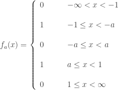
 . So we can consider
  . See
. See  , and for any open interval
 ![[x,(a,b)]=\left\{h \in C_p(\mathbb{S}): h(x) \in (a, b) \right\}](https://s0.wp.com/latex.php?latex=%5Bx%2C%28a%2Cb%29%5D%3D%5Cleft%5C%7Bh+%5Cin+C_p%28%5Cmathbb%7BS%7D%29%3A+h%28x%29+%5Cin+%28a%2C+b%29+%5Cright%5C%7D&bg=ffffff&fg=333333&s=0&c=20201002) . Then the collection of intersections of finitely many
. Then the collection of intersections of finitely many ![[x,(a,b)]](https://s0.wp.com/latex.php?latex=%5Bx%2C%28a%2Cb%29%5D&bg=ffffff&fg=333333&s=0&c=20201002) would form a base for
would form a base for  is a closed and discrete subspace of
 containing
  for any
  . To this end, let
 ![O=[a,V_1] \cap [-a,V_2]](https://s0.wp.com/latex.php?latex=O%3D%5Ba%2CV_1%5D+%5Ccap+%5B-a%2CV_2%5D&bg=ffffff&fg=333333&s=0&c=20201002) where
where  and
and  are the open intervals
  and
and  . With Figure 6 as an aid, it follows that for
  ,
,  and for
  ,
,  .
.  and
and  . Thus
  and
and  . Thus
  , there is an open set
  such that
  . As we consider
  such that
  .
.  and
and  . Then for all
  and for all
  . Let
. Let ![U=[a,(-0.1,0.1)] \cap [-a,(0.9,1.1)]](https://s0.wp.com/latex.php?latex=U%3D%5Ba%2C%28-0.1%2C0.1%29%5D+%5Ccap+%5B-a%2C%280.9%2C1.1%29%5D&bg=ffffff&fg=333333&s=0&c=20201002) . Then
. Then  and
and  for any
  for any
  and
and  has a similar argument.
 .
.  . Suppose not. Let
  such that
  . Suppose that
  . Consider
  . Clearly the number
  . Let
. Let  be a least upper bound of
  . Otherwise,
  would not be the least upper bound of the set
  in the interval
  such that
  from the left such that
  for all
  . Otherwise,
  . Otherwise, the function
  . By the assumption in Case 2,
  and
and  . Since
  for all
  from the right. Since
  , contradicting
  . Thus we cannot have
  where
where  . Clearly
  for all
  . Otherwise, the function
  and
and  . Since
  for all
 ![U=[0,(0.9,1.1)]](https://s0.wp.com/latex.php?latex=U%3D%5B0%2C%280.9%2C1.1%29%5D&bg=ffffff&fg=333333&s=0&c=20201002) . It is clear that
. It is clear that  . Let
. Let ![U=[-1,(-0.1,0.1)]](https://s0.wp.com/latex.php?latex=U%3D%5B-1%2C%28-0.1%2C0.1%29%5D&bg=ffffff&fg=333333&s=0&c=20201002) . It is clear that
. It is clear that  , then
  , the space of real-valued continuous functions defined on the number line with the pointwise convergence topology, is hereditarily separable and thus separable. Recall that continuous functions in
  be the set of all continuous functions from
  , let
, let  . Then
  . This representation is discussed
  is normal for all compact metric space
  if and only if
 ![W \times [0,1]](https://s0.wp.com/latex.php?latex=W+%5Ctimes+%5B0%2C1%5D&bg=ffffff&fg=333333&s=0&c=20201002) is normal. For the full statement of the theorem, see Theorem 1
is normal. For the full statement of the theorem, see Theorem 1  is normal,
 ![Y_x \times [0,1]](https://s0.wp.com/latex.php?latex=Y_x+%5Ctimes+%5B0%2C1%5D&bg=ffffff&fg=333333&s=0&c=20201002) is also normal. By Dowker’s theorem,
is also normal. By Dowker’s theorem,  is countably paracompact. Note that
  is normal for any
  -compact metric space
  . This means that
  is normal.
![(Y_x \times \mathbb{R}) \times [0,1]](https://s0.wp.com/latex.php?latex=%28Y_x+%5Ctimes+%5Cmathbb%7BR%7D%29+%5Ctimes+%5B0%2C1%5D&bg=ffffff&fg=333333&s=0&c=20201002) is normal. Thus according to Dowker’s theorem,
is normal. Thus according to Dowker’s theorem,  , one of the factors is perfectly normal or every countable subset of the other factor is closed (in that factor).
 ![[0,1]^X](https://s0.wp.com/latex.php?latex=%5B0%2C1%5D%5EX&bg=ffffff&fg=333333&s=0&c=20201002) has countable extent, hence is collectionwise normal (problem 294). See
has countable extent, hence is collectionwise normal (problem 294). See  is normal for any compact metric space
  is normal for any
  such that
  is an isolated point in
  is open in the subspace
  , a natural topology that can be given to
  . Let
. Let  . We say that
  is a limit point of
  if every open subset of
  on the space
  such that the diameters of the sets
  (based on the complete metric
  collapse to one point.
 such that
  . By assumption, both points are limit points of the space
  such that
  ,
, ,
, and
and  ,
, ,
, and
and  with respect to
  and
and  in the same manner. Before continuing, we set some notation. If
  and
and  (e.g. 01101 is extended by 011010 and 011011).
 is completed. This means that the points
  and the open sets
  have been chosen such that
  for each length
  st stage. For each
  and
and  and choose two open sets
  and
and  such that
 ,
, ,
, and
and  ,
, ,
, and
and  with respect to
  .
. , let
, let  be the union of all
  over all
  . Thus
  is non-empty. To complete the proof, we need to show that
  where
where  . Note that each element of
  is a countably infinite string of 0’s and 1’s. For each
  , let
, let  denote the string of the first
  . For each
  be the unique point in the following intersection:
 . At each next step, always pick the
  that matches the next digit of
  are two different strings of 0’s and 1’s, then they must differ at some coordinate, then from the way the induction is done, the strings would lead to two different points. It is also clear to see that the map
  . Then the point
  ‘s. This maps to a unique infinite string of 0’s and 1’s. Thus the set
  where
where  for all positive integers
  for each
  that are subsets of
  ). Because the diameters are decreasing to zero, the sequence of


 be the first uncountable ordinal, and let
  be the successor ordinal to
  such that the function
  . Now consider the function spaces
  and
and  . Thus individually, elements of these two function spaces appear identical. Any
  matches a function
  where
where  is the result of adding the point
  to
to  , is the least infinite cardinal
  such that for any
  , there exists
  for which
  and
and  . When
  , we say that
  , we say that
  . For each
  such that
  for all
  and
and  for all
  . Let
. Let  be the function that is identically zero. Then
  where
where  . It is clear that for any countable
  ,
,  . Thus
  is Lindelof for each
  .
. be a continuous surjection. Define a map
  by letting
  . It is shown in
  is a homeomorphism. Thus
  in
in  as a candidate for a homeomorphism between the two function spaces. The discussion in this post shows that this particular map is not a homeomorphism. In fact, no other one-to-one map from one of these function spaces onto the other function space can be a homeomorphism.
 . In fact,
 is the
  -product of
  be the following subspace of
 , i.e, the function space
  . On the other hand, the product
 be defined as follows:
 . Furthermore
  and is thus metrizable. Let
  for some
  is metrizable. The set
  is contained in
  , we have
  . A space
  . A longer discussion of the definition of monolithicity is found
  . A space
  .
. ![C_p([0,1])](https://s0.wp.com/latex.php?latex=C_p%28%5B0%2C1%5D%29&bg=ffffff&fg=333333&s=0&c=20201002) . It is clear that all metrizable spaces are strongly monolithic.
. It is clear that all metrizable spaces are strongly monolithic. , if
, if  , then there exists a sequence
  such that the sequence converges to
  , coincides with the network weight of
  . In [1],
  . The cardinal function
  , the weight of
  , since any continuous bijection from
  always holds. Thus
  . Thus we have:
 , then the cardinality of
 .
. by
by  for any
  . The map
  where
where  . Assume that
  . Then
  . So assume that
  . Then the functions
  and
and  are different, which means
  . Let
. Let  . Note that
  . Then
  . We have
  .
. is a matter of working with the basic open sets in the function space carefully (e.g. making the necessary shifting). Some authors just skip the details and declare them continuous, e.g. [1]. Readers are welcome to work out enough of the details to see the key idea.
 be an open set in
  and,
and, 

 are arbitrary points in
  is some large positive integer. Define the following:


 . We need to show
  . Let
. Let  . Then
  . We need to show that
  and
and  . Note that
  . For each
  ,
,  . So we have the following:


 . Hence
  . Let
. Let  be an open set in
  and
and

 of
of  and
and


 . Let
. Let  . We then have the following inequalities.

 ,
,  . It is clear that
  . Thus
  . This completes the proof that
  be a continuous surjection, i.e.,
  is a continuous function from
  by
by  for all
  . We show that
  with
with  . Choose some
  . Then
  since
since  and
and  .
. such that
 is an open interval of the real line
  ,
,  . Now consider the open set
  defined by:
 . It follows that
  since for each
  , it is clear that
  .
. is continuous. Let
  where
where  be open with
  such that
 are arbitrary points of
  is an open interval of
  such that
  for each
  for each
 . Note that
  . To see this, let
  where
where  . Now
. Now  for each
  . It follows that
  is continuous. The proof of the theorem is now complete.
  as follows:
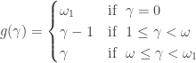
 where
where  . For each positive integer
  of
of  . Since
  such that
  for all
  . Because both
  and
and  with
with  such that
  for all
  . Let the open set
  be defined by
  . Let
. Let  .
. be countable such that
  is a cover of
  . Let
. Let  . Note that
  .
.  . Choose an arbitrary positive integer
  . Consider the open set
  .
.
 . Choose
  such that
  where
where  for all
  , leading to the conclusion that
 .
. , define
  by:
by:
 for each
  . We show that
  . We wish to establish the following claim. Once the claim is established, it follows that
  and
and  .
. . Case 2.
  .
. . Clearly
  for all
  , then consider the open set
  . Clearly
  . It is clear that no function in
  . Case 2.3.2.
  .
. . This
  such that
  . Case 2.3.2.2.
  for all
  . Note that
  for all
  . This means that
  . This is a contradiction since
  .
. where
where  . It is clear that
  . Furthermore,
  for all
  and
and  . Thus
  . This completes the proof that
  by
by  for all
  for all
  . Clearly
  and
and  . Furthermore,
  (the closure is taken in
  . Let
. Let  .
.  that takes on the constant value of 1. It follows that
  (the closure is in