(Lower case) sigma-products of separable metric spaces are Lindelof

Consider the product space X=\prod_{\alpha \in A} X_\alpha. Fix a point b \in \prod_{\alpha \in A} X_\alpha, called the base point. The \Sigma-product of the spaces \left\{X_\alpha: \alpha \in A \right\} is the following subspace of the product space X:

    \Sigma_{\alpha \in A} X_\alpha=\left\{ x \in X: x_\alpha \ne b_\alpha \text{ for at most countably many } \alpha \in A \right\}

In other words, the space \Sigma_{\alpha \in A} X_\alpha is the subspace of the product space X=\prod_{\alpha \in A} X_\alpha consisting of all points that deviate from the base point on at most countably many coordinates \alpha \in A. We also consider the following subspace of \Sigma_{\alpha \in A} X_\alpha.

    \sigma=\left\{ x \in \Sigma_{\alpha \in A} X_\alpha: x_\alpha \ne b_\alpha \text{ for at most finitely many } \alpha \in A \right\}

For convenience , we call \Sigma_{\alpha \in A} X_\alpha the (upper case) Sigma-product (or \Sigma-product) of the spaces X_\alpha and we call the space \sigma the (lower case) sigma-product (or \sigma-product). Clearly, the space \sigma is a dense subspace of \Sigma_{\alpha \in A} X_\alpha. In a previous post, we show that the upper case Sigma-product of separable metric spaces is collectionwise normal. In this post, we show that the (lower case) sigma-product of separable metric spaces is Lindelof. Thus when each factor X_\alpha is a separable metric space with at least two points, the \Sigma-product, though not Lindelof, has a dense Lindelof subspace. The (upper case) \Sigma-product of separable metric spaces is a handy example of a non-Lindelof space that contains a dense Lindelof subspace.

Naturally, the lower case sigma-product can be further broken down into countably many subspaces. For each integer n=0,1,2,3,\cdots, we define \sigma_n as follows:

    \sigma_n=\left\{ x \in \sigma: x_\alpha \ne b_\alpha \text{ for at most } n \text{ many } \alpha \in A \right\}

Clearly, \sigma=\bigcup_{n=0}^\infty \sigma_n. We prove the following theorem. The fact that \sigma is Lindelof will follow as a corollary. Understanding the following proof for Theorem 1 is a matter of keeping straight the notations involving standard basic open sets in the product space X=\prod_{\alpha \in A} X_\alpha. We say V is a standard basic open subset of the product space X if V is of the form V=\prod_{\alpha \in A} V_\alpha such that each V_\alpha is an open subset of the factor space X_\alpha and V_\alpha=X_\alpha for all but finitely many \alpha \in A. The finite set F of all \alpha \in A such that V_\alpha \ne X_\alpha is called the support of the open set V.

Theorem 1
Let \sigma be the \sigma-product of the separable metrizable spaces \left\{X_\alpha: \alpha \in A \right\}. For each n, let \sigma_n be defined as above. The product space \sigma_n \times Y is Lindelof for each non-negative integer n and for all separable metric space Y.

Proof of Theorem 1
We prove by induction on n. Note that \sigma_0=\left\{b \right\}, the base point. Clearly \sigma_0 \times Y is Lindelof for all separable metric space Y. Suppose the theorem hold for the integer n. We show that \sigma_{n+1} \times Y for all separable metric space Y. To this end, let \mathcal{U} be an open cover of \sigma_{n+1} \times Y where Y is a separable metric space. Without loss of generality, we assume that each element of \mathcal{U} is of the form V \times W where V=\prod_{\alpha \in A} V_\alpha is a standard basic open subset of the product space X=\prod_{\alpha \in A} X_\alpha and W is an open subset of Y.

Let \mathcal{U}_0=\left\{U_1,U_2,U_3,\cdots \right\} be a countable subcollection of \mathcal{U} such that \mathcal{U}_0 covers \left\{b \right\} \times Y. For each j, let U_j=V_j \times W_j where V_j=\prod_{\alpha \in A} V_{j,\alpha} is a standard basic open subset of the product space X with b \in V_j and W_j is an open subset of Y. For each j, let F_j be the support of V_j. Note that \alpha \in F_j if and only if V_{j,\alpha} \ne X_\alpha. Also for each \alpha \in F_j, b_\alpha \in V_{j,\alpha}. Furthermore, for each \alpha \in F_j, let V^c_{j,\alpha}=X_\alpha- V_{j,\alpha}. With all these notations in mind, we define the following open set for each \beta \in F_j:

    H_{j,\beta}= \biggl( V^c_{j,\beta} \times \prod_{\alpha \in A, \alpha \ne \beta} X_\alpha \biggr) \times W_j=\biggl( V^c_{j,\beta} \times T_\beta \biggr) \times W_j

Observe that for each point y \in \sigma_{n+1} such that y \in V^c_{j,\beta} \times T_\beta, the point y already deviates from the base point b on one coordinate, namely \beta. Thus on the coordinates other than \beta, the point y can only deviates from b on at most n many coordinates. Thus \sigma_{n+1} \cap (V^c_{j,\beta} \times T_\beta) is homeomorphic to V^c_{j,\beta} \times \sigma_n. Note that V^c_{j,\beta} \times W_j is a separable metric space. By inductive hypothesis, V^c_{j,\beta} \times \sigma_n \times W_j is Lindelof. Thus there are countably many open sets in the open cover \mathcal{U} that covers points of H_{j,\beta} \cap (\sigma_{n+1} \times W_j).

Note that

    \sigma_{n+1} \times Y=\biggl( \bigcup_{j=1}^\infty U_j \cap \sigma_{n+1} \biggr) \cup \biggl( \bigcup \left\{H_{j,\beta} \cap (\sigma_{n+1} \times W_j): j=1,2,3,\cdots, \beta \in F_j \right\} \biggr)

To see that the left-side is a subset of the right-side, let t=(x,y) \in \sigma_{n+1} \times Y. If t \in U_j for some j, we are done. Suppose t \notin U_j for all j. Observe that y \in W_j for some j. Since t=(x,y) \notin U_j, x_\beta \notin V_{j,\beta} for some \beta \in F_j. Then t=(x,y) \in H_{j,\beta}. It is now clear that t=(x,y) \in H_{j,\beta} \cap (\sigma_{n+1} \times W_j). Thus the above set equality is established. Thus one part of \sigma_{n+1} \times Y is covered by countably many open sets in \mathcal{U} while the other part is the union of countably many Lindelof subspaces. It follows that a countable subcollection of \mathcal{U} covers \sigma_{n+1} \times Y. \blacksquare

Corollary 2
It follows from Theorem 1 that

  • If each factor space X_\alpha is a separable metric space, then each \sigma_n is a Lindelof space and that \sigma=\bigcup_{n=0}^\infty \sigma_n is a Lindelof space.
  • If each factor space X_\alpha is a compact separable metric space, then each \sigma_n is a compact space and that \sigma=\bigcup_{n=0}^\infty \sigma_n is a \sigma-compact space.

Proof of Corollary 2
The first bullet point is a clear corollary of Theorem 1. A previous post shows that \Sigma-product of compact spaces is countably compact. Thus \Sigma_{\alpha \in A} X_\alpha is a countably compact space if each X_\alpha is compact. Note that each \sigma_n is a closed subset of \Sigma_{\alpha \in A} X_\alpha and is thus countably compact. Being a Lindelof space, each \sigma_n is compact. It follows that \sigma=\bigcup_{n=0}^\infty \sigma_n is a \sigma-compact space. \blacksquare

____________________________________________________________________

A non-Lindelof space with a dense Lindelof subspace

Now we put everything together to obtain the example described at the beginning. For each \alpha \in A, let X_\alpha be a separable metric space with at least two points. Then the \Sigma-product \Sigma_{\alpha \in A} X_\alpha is collectionwise normal (see this previous post). According to the lemma in this previous post, the \Sigma-product \Sigma_{\alpha \in A} X_\alpha contains a closed copy of \omega_1. Thus the \Sigma-product \Sigma_{\alpha \in A} X_\alpha is not Lindelof. It is clear that the \sigma-product is a dense subspace of \Sigma_{\alpha \in A} X_\alpha. By Corollary 2, the \sigma-product is a Lindelof subspace of \Sigma_{\alpha \in A} X_\alpha.

Using specific factor spaces, if each X_\alpha=\mathbb{R} with the usual topology, then \Sigma_{\alpha<\omega_1} X_\alpha is a non-Lindelof space with a dense Lindelof subspace. On the other hand, if each X_\alpha=[0,1] with the usual topology, then \Sigma_{\alpha<\omega_1} X_\alpha is a non-Lindelof space with a dense \sigma-compact subspace. Another example of a non-Lindelof space with a dense Lindelof subspace is given In this previous post (see Example 1).

____________________________________________________________________

\copyright \ 2014 \text{ by Dan Ma}

Normal dense subspaces of products of “omega 1” many separable metric factors

Is every normal dense subspace of a product of separable metric spaces collectionwise normal? This question was posed by Arkhangelskii (see Problem I.5.25 in [2]). One partial positive answer is a theorem attributed to Corson: if Y is a normal dense subspace of a product of separable spaces such that Y \times Y is normal, then Y is collectionwise normal. Another partial positive answer: assuming 2^\omega<2^{\omega_1}, any normal dense subspace of the product space of continuum many separable metric factors is collectionwise normal (see Corollary 4 in this previous post). Another partial positive answer to Arkhangelskii’s question is the theorem due to Reznichenko: If C_p(X), which is a dense subspace of the product space \mathbb{R}^X, is normal, then it is collectionwise normal (see Theorem I.5.12 in [2]). In this post, we highlight another partial positive answer to the question posted in [2]. Specifically, we prove the following theorem:

Theorem 1

    Let X=\prod_{\alpha<\omega_1} X_\alpha be a product space where each factor X_\alpha is a separable metric space. Let Y be a dense subspace of X. Then if Y is normal, then Y is collectionwise normal.

Since any normal space with countable extent is collectionwise normal (see Theorem 2 in this previous post), it suffices to prove the following theorem:

Theorem 1a

    Let X=\prod_{\alpha<\omega_1} X_\alpha be a product space where each factor X_\alpha is a separable metric space. Let Y be a dense subspace of X. Then if Y is normal, then every closed and discrete subspace of Y is countable, i.e., Y has countable extent.

Arkhangelskii’s question was studied by the author of [3] and [4]. Theorem 1 as presented in this post is essentially the Theorem 1 found in [3]. The proof given in [3] is a beautiful proof. The proof in this post is modeled on the proof in [3] with the exception that all the crucial details are filled in. Theorem 1a (as stated above) is used in [1] to show that the function space C_p(\omega_1+1) contains no dense normal subspace.

It is natural to wonder if Theorem 1 can be generalized to product space of \tau many separable metric factors where \tau is an arbitrary uncountable cardinal. The work of [4] shows that the question at the beginning of this post cannot be answered positively in ZFC. Recall the above mentioned result that assuming 2^\omega<2^{\omega_1}, any normal dense subspace of the product space of continuum many separable metric factors is collectionwise normal (see Corollary 4 in this previous post). A theorem in [4] implies that assuming 2^\omega=2^{\omega_1}, for any separable metric space M with at least 2 points, the product of continuum many copies of M contains a normal dense subspace Y that is not collectionwise normal. A side note: for this normal subspace Y, Y \times Y is necessarily not normal (according to Corson’s theorem). Thus [3] and [4] collectively show that Arkhangelskii’s question stated here at the beginning of the post is answered positively (in ZFC) among product spaces of \omega_1 many separable metric factors and that outside of the \omega_1 case, it is impossible to answer the question positively in ZFC.

____________________________________________________________________

Proving Theorem 1a

We use the following lemma. For a proof of this lemma, see the proof for Lemma 1 in this previous post.

Lemma 2

    Let X=\prod_{\alpha \in A} X_\alpha be a product of separable metrizable spaces. Let Y be a dense subspace of X. Then the following conditions are equivalent.

    1. Y is normal.
    2. For any pair of disjoint closed subsets H and K of Y, there exists a countable B \subset A such that \overline{\pi_B(H)} \cap \overline{\pi_B(K)}=\varnothing.
    3. For any pair of disjoint closed subsets H and K of Y, there exists a countable B \subset A such that \pi_B(H) and \pi_B(K) are separated in \pi_B(Y), meaning that \overline{\pi_B(H)} \cap \pi_B(K)=\pi_B(H) \cap \overline{\pi_B(K)}=\varnothing.

For any B \subset \omega_1, let \pi_B be the natural projection from the product space X=\prod_{\alpha<\omega_1} X_\alpha into the subproduct space \prod_{\alpha \in B} X_\alpha.

Proof of Theorem 1a
Let Y be a dense subspace of the product space X=\prod_{\alpha<\omega_1} X_\alpha where each factor X_\alpha has a countable base. Suppose that D is an uncountable closed and discrete subset of Y. We then construct a pair of disjoint closed subsets H and K of Y such that for all countable B \subset \omega_1, \pi_B(H) and \pi_B(K) are not separated, specifically \pi_B(H) \cap \overline{\pi_B(K)}\ne \varnothing. Here the closure is taken in the space \pi_B(Y). By Lemma 2, the dense subspace Y of X is not normal.

For each \alpha<\omega_1, let \mathcal{B}_\alpha be a countable base for the space X_\alpha. The standard basic open sets in the product space X are of the form O=\prod_{\alpha<\omega_1} O_\alpha such that

  • each O_\alpha is an open subset of X_\alpha,
  • if O_\alpha \ne X_\alpha, then O_\alpha \in \mathcal{B}_\alpha,
  • O_\alpha=X_\alpha for all but finitely many \alpha<\omega_1.

We use supp(O) to denote the finite set of \alpha such that O_\alpha \ne X_\alpha. Technically we should be working with standard basic open subsets of Y, i.e., sets of the form O \cap Y where O is a standard basic open set as described above. Since Y is dense in the product space, every standard open set contains points of Y. Thus we can simply work with standard basic open sets in the product space as long as we are working with points of Y in the construction.

Let \mathcal{M} be the collection of all standard basic open sets as described above. Since there are only \omega_1 many factors in the product space, \lvert \mathcal{M} \lvert=\omega_1. Recall that D is an uncountable closed and discrete subset of Y. Let \mathcal{M}^* be the following:

    \mathcal{M}^*=\left\{U \in \mathcal{M}: U \cap D \text{ is uncountable }  \right\}

Claim 1. \lvert \mathcal{M}^* \lvert=\omega_1.

First we show that \mathcal{M}^* \ne \varnothing. Let B \subset \omega_1 be countable. Consider these two cases: Case 1. \pi_B(D) is an uncountable subset of \prod_{\alpha \in B} X_\alpha; Case 2. \pi_B(D) is countable.

Suppose Case 1 is true. Since \prod_{\alpha \in B} X_\alpha is a product of countably many separable metric spaces, it is hereditarily Lindelof. Then there exists a point y \in \pi_B(D) such that every open neighborhood of y (open in \prod_{\alpha \in B} X_\alpha) contains uncountably many points of \pi_B(D). Thus every standard basic open set U=\prod_{\alpha \in B} U_\alpha, with y \in U, contains uncountably many points of \pi_B(D). Suppose Case 2 is true. There exists one point y \in \pi_B(D) such that y=\pi_B(t) for uncountably many t \in D. Then in either case, every standard basic open set V=\prod_{\alpha<\omega_1} V_\alpha, with supp(V) \subset B and y \in \pi_B(V), contains uncountably many points of D. Any one such V is a member of \mathcal{M}^*.

We can partition the index set \omega_1 into \omega_1 many disjoint countable sets B. Then for each such B, obtain a V \in \mathcal{M}^* in either Case 1 or Case 2. Since supp(V) \subset B, all such open sets V are distinct. Thus Claim 1 is established.

Claim 2.
There exists an uncountable H \subset D such that for each U \in \mathcal{M}^*, U \cap H \ne \varnothing and U \cap (D-H) \ne \varnothing.

Enumerate \mathcal{M}^*=\left\{U_\gamma: \gamma<\omega_1 \right\}. Choose h_0,k_0 \in U_0 \cap D with h_0 \ne k_0. Suppose that for all \beta<\gamma, two points h_\beta,k_\beta are chosen such that h_\beta,k_\beta \in U_\beta \cap D, h_\beta \ne k_\beta and such that h_\beta \notin L_\beta and k_\beta \notin L_\beta where L_\beta=\left\{h_\rho: \rho<\beta \right\} \cup \left\{k_\rho: \rho<\beta \right\}. Then choose h_\gamma,k_\gamma with h_\gamma \ne k_\gamma such that h_\gamma,k_\gamma \in U_\gamma \cap D and h_\gamma \notin L_\gamma and k_\gamma \notin L_\gamma where L_\gamma=\left\{h_\rho: \rho<\gamma \right\} \cup \left\{k_\rho: \rho<\gamma \right\}.

Let H=\left\{h_\gamma: \gamma<\omega_1 \right\} and let K=D-H. Note that K_0=\left\{k_\gamma: \gamma<\omega_1 \right\} \subset K. Based on the inductive process that is used to obtain H and K_0, it is clear that H satisfies Claim 2.

Claim 3.
For each countable B \subset \omega_1, the sets \pi_B(H) and \pi_B(K) are not separated in the space \pi_B(Y).

Let B \subset \omega_1 be countable. Consider the two cases: Case 1. \pi_B(H) is uncountable; Case 2. \pi_B(H) is countable. Suppose Case 1 is true. Since \prod_{\alpha \in B} X_\alpha is a product of countably many separable metric spaces, it is hereditarily Lindelof. Then there exists a point p \in \pi_B(H) such that every open neighborhood of p (open in \prod_{\alpha \in B} X_\alpha) contains uncountably many points of \pi_B(H). Choose h \in H such that p=\pi_B(h). Then the following statement holds:

  1. For every basic open set U=\prod_{\alpha<\omega_1} U_\alpha with h \in U such that supp(U) \subset B, the open set U contains uncountably many points of H.

Suppose Case 2 is true. There exists some p \in \pi_B(H) such that p=\pi_B(t) for uncountably many t \in H. Choose h \in H such that p=\pi_B(h). Then statement 1 also holds.

In either case, there exists h \in H such that statement 1 holds. The open sets U described in statement 1 are members of \mathcal{M}^*. By Claim 2, the open sets described in statement 1 also contain points of K. Since the open sets described in statement 1 have supports \subset B, the following statement holds:

  1. For every basic open set V=\prod_{\alpha \in B} V_\alpha with \pi_B(h) \in V, the open set V contains points of \pi_B(K).

Statement 2 indicates that \pi_B(h) \in \overline{\pi_B(K)}. Thus \pi_B(h) \in \pi_B(H) \cap \overline{\pi_B(K)}. The closure here can be taken in either \prod_{\alpha \in B} X_\alpha or \pi_B(Y) (to apply Lemma 2, we only need the latter). Thus Claim 3 is established.

Claim 3 is the negation of condition 3 of Lemma 2. Therefore Y is not normal. \blacksquare

____________________________________________________________________

Remark

The proof of Theorem 1a, though a proof in ZFC only, clearly relies on the fact that the product space is a product of \omega_1 many factors. For example, in the inductive step in the proof of Claim 2, it is always possible to pick a pair of points not chosen previously. This is because the previously chosen points form a countable set and each open set in \mathcal{M}^* contains \omega_1 many points of the closed and discrete set D. With the “\omega versus \omega_1” situation, at each step, there are always points not previously chosen. When more than \omega_1 many factors are involved, there may be no such guarantee in the inductive process.

____________________________________________________________________

Reference

  1. Arkhangelskii, A. V., Normality and dense subspaces, Proc. Amer. Math. Soc., 130 (1), 283-291, 2001.
  2. Arkhangelskii, A. V., Topological Function Spaces, Mathematics and Its Applications Series, Kluwer Academic Publishers, Dordrecht, 1992.
  3. Baturov, D. P., Normality in dense subspaces of products, Topology Appl., 36, 111-116, 1990.
  4. Baturov, D. P., On perfectly normal dense subspaces of products, Topology Appl., 154, 374-383, 2007.
  5. Engelking, R., General Topology, Revised and Completed edition, Heldermann Verlag, Berlin, 1989.

____________________________________________________________________

\copyright \ 2014 \text{ by Dan Ma}

Normal dense subspaces of a product of “continuum” many separable metric factors

Is every normal dense subspace of a product of separable metric spaces collectionwise normal? This question was posed by Arkhangelskii in [1] (see Problem I.5.25). A partial positive answer is provided by a theorem that is usually attributed to Corson: If Y is a normal dense subspace of a product of separable metric spaces and if Y \times Y is also normal, then Y is collectionwise normal. In this post, using a simple combinatorial argument, we show that any normal dense subspace of a product of continuum many separable metric space is collectionwise normal (see Corollary 4 below), which is a corollary of the following theorem.

Theorem 1
Let X be a normal space with character \le 2^\omega. If 2^\omega<2^{\omega_1}, then the following holds:

  • If Y is a closed and discrete subspace of X with \lvert Y \lvert=\omega_1, then Y contains a separated subset of cardinality \omega_1.

Theorem 1 gives the corollary indicated at the beginning and several other interesting results. The statement 2^\omega<2^{\omega_1} means that the cardinality of the power set (the set of all subsets) of \omega is strictly less than the cardinality of the power set of \omega_1. Note that the statement 2^\omega<2^{\omega_1} follows from the continuum hypothesis (CH), the statement that 2^\omega=\omega_1. With the assumption 2^\omega<2^{\omega_1}, Theorem 1 is a theorem that goes beyond ZFC. We also present an alternative to Theorem 1 that removes the assumption 2^\omega<2^{\omega_1} (see Theorem 6 below).

A subset T of a space S is a separated set (in S) if for each t \in T, there is an open subset O_t of S with t \in O_t such that \left\{O_t: t \in T \right\} is a pairwise disjoint collection. First we prove Theorem 1 and then discuss the corollaries.

____________________________________________________________________

Proof of Theorem 1

Suppose Y is a closed and discrete subset of X with \lvert Y \lvert=\omega_1 such that no subset of Y of cardinality \omega_1 can be separated. We then show that 2^{\omega_1} \le 2^{\omega}.

For each y \in Y, let \mathcal{B}_y be a local base at the point y such that \lvert \mathcal{B}_y \lvert \le 2^\omega. Let \mathcal{B}=\bigcup_{y \in Y} \mathcal{B}_y. Thus \lvert \mathcal{B} \lvert \le 2^\omega. By normality, for each W \subset Y, let U_W be an open subset of X such that W \subset U_W and \overline{U_W} \cap (Y-W)=\varnothing. For each W \subset Y, consider the following collection of open sets:

    \mathcal{G}_W=\left\{V \in \mathcal{B}_y: y \in W \text{ and } V \subset U_W  \right\}

For each W \subset Y, choose a maximal disjoint collection \mathcal{M}_W of open sets in \mathcal{G}_W. Because no subset of Y of cardinality \omega_1 can be separated, each \mathcal{M}_W is countable. If W_1 \ne W_2, then \mathcal{M}_{W_1} \ne \mathcal{M}_{W_2}.

Let \mathcal{P}(Y) be the power set (i.e. the set of all subsets) of Y. Let \mathcal{P}_\omega(\mathcal{B}) be the set of all countable subsets of \mathcal{B}. Then the mapping W \mapsto \mathcal{M}_W is a one-to-one map from \mathcal{P}(Y) into \mathcal{P}_\omega(\mathcal{B}). Note that \lvert \mathcal{P}(Y) \lvert=2^{\omega_1}. Also note that since \lvert \mathcal{B} \lvert \le 2^\omega, \lvert \mathcal{P}_\omega(\mathcal{B}) \lvert \le 2^\omega. Thus 2^{\omega_1} \le 2^{\omega}. \blacksquare

____________________________________________________________________

Some Corollaries of Theorem 1

Here’s some corollaries that follow easily from Theorem 1. A space X has the countable chain condition (CCC) if every pairwise disjoint collection of non-empty open subset of X is countable. For convenience, if X has the CCC, we say X is CCC. The following corollaries make use of the fact that any normal space with countable extent is collectionwise normal (see Theorem 2 in this previous post).

Corollary 2
Let X be a CCC space with character \le 2^\omega. If 2^\omega<2^{\omega_1}, then the following conditions hold:

  • If X is normal, then every closed and discrete subset of X is countable, i.e., X has countable extent.
  • If X is normal, then X is collectionwise normal.

Corollary 3
Let X be a CCC space with character \le 2^\omega. If CH holds, then the following conditions hold:

  • If X is normal, then every closed and discrete subset of X is countable, i.e., X has countable extent.
  • If X is normal, then X is collectionwise normal.

Corollary 4
Let X=\prod_{\alpha<2^\omega} X_\alpha be a product where each factor X_\alpha is a separable metric space. If 2^\omega<2^{\omega_1}, then the following conditions hold:

  • If Y is a normal dense subspace of X, then Y has countable extent.
  • If Y is a normal dense subspace of X, then Y is collectionwise normal.

Corollary 4 is the result indicated in the title of the post. The product of separable spaces has the CCC. Thus the product space X and any dense subspace of X have the CCC. Because X is a product of continuum many separable metric spaces, X and any subspace of X have characters \le 2^\omega. Then Corollary 4 follows from Corollary 2.

When dealing with the topic of normal versus collectionwise normal, it is hard to avoid the connection with the normal Moore space conjecture. Theorem 1 gives the result of F. B. Jones from 1937 (see [3]). We have the following theorem.

Theorem 5
If 2^\omega<2^{\omega_1}, then every separable normal Moore space is metrizable.

Though this was not how Jones proved it in [3], Theorem 5 is a corollary of Corollary 2. By Corollary 2, any separable normal Moore space is collectionwise normal. It is well known that collectionwise normal Moore space is metrizable (Bing’s metrization theorem, see Theorem 5.4.1 in [2]).

____________________________________________________________________

A ZFC Theorem

We now prove a result that is similar to Corollary 2 but uses no set-theory beyond the Zermelo–Fraenkel set theory plus axiom of choice (abbreviated by ZFC). Of course the conclusion is not as strong. Even though the assumption 2^\omega<2^{\omega_1} is removed in Theorem 6, note the similarity between the proof of Theorem 1 and the proof of Theorem 6.

Theorem 6
Let X be a CCC space with character \le 2^\omega. Then the following conditions hold:

  • If X is normal, then every closed and discrete subset of X has cardinality less than continuum.

Proof of Theorem 6
Let X be a normal CCC space with character \le 2^\omega. Let Y be a closed and discrete subset of X. We show that \lvert Y \lvert < 2^\omega. Suppose that \lvert Y \lvert = 2^\omega.

For each y \in Y, let \mathcal{B}_y be a local base at the point y such that \lvert \mathcal{B}_y \lvert \le 2^\omega. Let \mathcal{B}=\bigcup_{y \in Y} \mathcal{B}_y. Thus \lvert \mathcal{B} \lvert = 2^\omega. By normality, for each W \subset Y, let U_W be an open subset of X such that W \subset U_W and \overline{U_W} \cap (Y-W)=\varnothing. For each W \subset Y, consider the following collection of open sets:

    \mathcal{G}_W=\left\{V \in \mathcal{B}_y: y \in W \text{ and } V \subset U_W  \right\}

For each W \subset Y, choose \mathcal{M}_W \subset \mathcal{G}_W such that \mathcal{M}_W is a maximal disjoint collection. Since X is CCC, \mathcal{M}_W is countable. It is clear that if W_1 \ne W_2, then \mathcal{M}_{W_1} \ne \mathcal{M}_{W_2}.

Let \mathcal{P}(Y) be the power set (i.e. the set of all subsets) of Y. Let \mathcal{P}_\omega(\mathcal{B}) be the set of all countable subsets of \mathcal{B}. Then the mapping W \mapsto \mathcal{M}_W is a one-to-one map from \mathcal{P}(Y) into \mathcal{P}_\omega(\mathcal{B}). Note that since \lvert \mathcal{B} \lvert = 2^\omega, \lvert \mathcal{P}_\omega(\mathcal{B}) \lvert = 2^\omega. Thus \lvert \mathcal{P}(Y) \lvert \le 2^{\omega}. However, Y is assumed to be of cardinality continuum. Then \lvert \mathcal{P}(Y) \lvert>2^{\omega_1}, leading to a contradiction. Thus it must be the case that \lvert Y \lvert < 2^\omega. \blacksquare

With Theorem 6, Corollary 3 still holds. Theorem 6 removes the set-theoretic assumption of 2^\omega<2^{\omega_1}. As a result, the upper bound for cardinalities of closed and discrete sets is (at least potentially) higher.

____________________________________________________________________

Reference

  1. Arkhangelskii, A. V., Topological Function Spaces, Mathematics and Its Applications Series, Kluwer Academic Publishers, Dordrecht, 1992.
  2. Engelking, R., General Topology, Revised and Completed edition, Heldermann Verlag, Berlin, 1989.
  3. Jones, F. B., Concerning normal and completely normal spaces, Bull. Amer. Math. Soc., 43, 671-677, 1937.

____________________________________________________________________

\copyright \ 2014 \text{ by Dan Ma}

Looking for another closed and discrete subspace of a product space

Let \omega_1 be the first uncountable ordinal. In a previous post called Looking for a closed and discrete subspace of a product space, it was shown that the product space \mathbb{R}^c, the product of continuum many copies of the real line \mathbb{R}, contains a closed and discrete subset of cardinality continuum. This example shows that a product space of uncountably many copies of a “nice” space is “big and wide” enough to hide uncountable closed and discrete sets even when the product space is separable. This post reinforces this same fact by showing that \mathbb{R}^{\omega_1} contains a closed and discrete subset of cardinality \omega_1. It follows that for any uncountable cardinal \tau, the product space \mathbb{R}^\tau contains an uncountable closed and discrete subset, i.e., the product of uncountably many copies of the real line \mathbb{R} has uncountable extent.

Let \omega be the first infinite ordinal, i.e., the set of all nonnegative integers. Consider \omega^{\omega_1}, the product of \omega_1 many copies of \omega with the discrete topology. Since \omega^{\omega_1} is a closed subspace of \mathbb{R}^{\omega_1}, it suffices to show that \omega^{\omega_1} has an uncountable closed and discrete subset.

____________________________________________________________________

The Construction

We now construct an uncountable closed and discrete subset of \omega^{\omega_1}. Let \delta be an infinite ordinal such that \omega<\delta<\omega_1. Let W=\left\{\alpha: \delta \le \alpha<\omega_1 \right\}. For each \alpha \in W, let Y_\alpha=\left\{\beta<\omega_1: \beta<\alpha \right\}. We can also use interval notations: W=[\delta,\omega_1) and Y_\alpha=[0,\alpha). Consider Y_\alpha as a space with the discrete topology. Then it is clear that \omega^{\omega_1} is homeomorphic to the product space \prod_{\alpha \in W} Y_\alpha. Thus the focus is now on finding an uncountable closed and discrete subset of \prod_{\alpha \in W} Y_\alpha.

One interesting fact about the space \prod_{\alpha \in W} Y_\alpha is that every function f \in \prod_{\alpha \in W} Y_\alpha is a pressing down function. That is, for every f \in \prod_{\alpha \in W} Y_\alpha, f(\alpha)<\alpha for all \alpha \in W. Note that f is defined on W, a closed and unbounded subset of \omega_1 (hence a stationary set). It follows that for each f \in \prod_{\alpha \in W} Y_\alpha, there is a stationary set S \subset W and there exists \rho<\omega_1 such that f(\alpha)=\rho for all \alpha \in S. This fact is called the pressing down lemma and will be used below. See this post for more information about the pressing down lemma.

For each \gamma \in W, let h_\gamma: Y_{\gamma+1} \rightarrow \delta be a one-to-one function. For each \gamma \in W, define t_\gamma \in \prod_{\alpha \in W} Y_\alpha as follows:

    t_\gamma(\alpha) = \begin{cases} h_\gamma(\alpha) & \mbox{if } \delta \le \alpha \le \gamma \\ \gamma & \mbox{if } \gamma < \alpha <\omega_1  \end{cases}

Note that each t_\gamma 
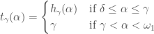
is a pressing down function. Thus each t_\gamma \in \prod_{\alpha \in W} Y_\alpha. Let T=\left\{t_\gamma: \gamma \in W \right\}. Clearly t_\gamma \ne t_\mu if \gamma \ne \mu. Thus T has cardinality \omega_1. We claim that T is a closed and discrete subset of \prod_{\alpha \in W} Y_\alpha. It suffices to show that for each f \in \prod_{\alpha \in W} Y_\alpha, there exists an open set V with f \in V such that V contains at most one t_\gamma.

Let f \in \prod_{\alpha \in W} Y_\alpha. As discussed above, there is a stationary set S \subset W and there exists \rho<\omega_1 such that f(\alpha)=\rho for all \alpha \in S. In particular, choose \mu, \lambda \in S such that \mu \ne \lambda. Thus f(\mu)=f(\lambda)=\rho. Let V be the open set defined by:

    V=\left\{g \in \prod_{\alpha \in W} Y_\alpha: g(\mu)=g(\lambda)=\rho \right\}

Clearly, f \in V. We show that if t_\gamma \in V, then \gamma=\rho. Suppose t_\gamma \in V. Then t_\gamma(\mu)=t_\gamma(\lambda)=\rho. Consider two cases: Case 1: \delta \le \mu, \lambda \le \gamma; Case 2: one of \mu and \lambda>\gamma. The definition of t_\gamma indicates that t_\gamma=h_\gamma on the interval [\delta, \gamma]. Note that h_\gamma is a one-to-one function. Since t_\gamma(\mu)=t_\gamma(\lambda), it cannot be that \mu, \lambda \in [\delta, \gamma], i.e., Case 1 is not possible. Thus Case 2 holds, say \mu>\gamma. Then by definition, t_\gamma(\mu)=\gamma. Putting everything together, \gamma=t_\gamma(\mu)=t_\gamma(\lambda)=\rho. Thus V \cap T \subset \left\{t_\rho \right\}. This concludes the proof that the set T is a closed and discrete subset of \prod_{\alpha \in W} Y_\alpha. \blacksquare

____________________________________________________________________

\copyright \ 2014 \text{ by Dan Ma}

Sigma-products of first countable spaces

A product space is never first countable if there are uncountably many factors. For example, \prod_{\alpha < \omega_1}\mathbb{R}=\mathbb{R}^{\omega_1} is not first countable. In fact any dense subspace of \mathbb{R}^{\omega_1} is not first countable. In particular, the subspace of \mathbb{R}^{\omega_1} consisting of points which have at most countably many non-zero coordinates is not first countable. This subspace is called the \Sigma-product of \omega_1 many copies of the real line \mathbb{R} and is denoted by \Sigma_{\alpha<\omega_1} \mathbb{R}. However, this \Sigma-product is a Frechet space (or a Frechet-Urysohn space). In this post, we show that the \Sigma-product of first countable spaces is a Frechet space.

Consider the product space X=\prod_{\alpha \in A} X_\alpha. Fix a point a \in X. Consider the following subspace of X:

    \Sigma_{\alpha \in A} X_\alpha(a)=\left\{x \in X: x_\alpha \ne a_\alpha \text{ for at most countably many } \alpha \in A \right\}

The above subspace of X is called the \Sigma-product of the spaces \left\{X_\alpha: \alpha \in A \right\} about the base point a. When the base point is understood, we simply say the \Sigma-product of the spaces \left\{X_\alpha: \alpha \in A \right\} and use the notation \Sigma_{\alpha \in A} X_\alpha to denote the space.

For each y \in \Sigma_{\alpha \in A} X_\alpha, define S(y) to be the set of all \alpha \in A such that y_\alpha \ne a_\alpha, i.e., the support of the point y. Another notion of support is that of standard basic open sets in the product topology. A standard basic open set is a set O=\prod_{\alpha \in A} O_\alpha where each O_\alpha is an open subset of X_\alpha. The support of O, denoted by supp(O) is the finite set of all \alpha \in A such that O_\alpha \ne X_\alpha.

A space Y is said to be first countable if there exists a countable local base at each point in Y. A space Y is said to be a Frechet space if for each y \in Y and for each M \subset Y, if y \in \overline{M}, then there exists a sequence \left\{y_n: n=1,2,3,\cdots \right\} of points of M such that the sequence converges to y. Frechet spaces also go by the name of Frechet-Urysohn spaces. Clearly, any first countable space is Frechet. The converse is not true (see Example 1 in this post). We prove the following theorem.

Theorem 1

    Suppose each factor X_\alpha is a first countable space. Then the \Sigma-product \Sigma_{\alpha \in A} X_\alpha is a Frechet space.

Proof of Theorem 1
Let \Sigma=\Sigma_{\alpha \in A} X_\alpha. Let M \subset \Sigma and let x \in \overline{M}. We proceed to define a sequence of points t_n \in M such that the sequence t_n converges to x. For each \alpha \in A, choose a countable local base \left\{B_{\alpha,j}: j=1,2,3,\cdots \right\} at the point x_\alpha \in X_\alpha. Assume that B_{\alpha,1} \supset B_{\alpha,2} \supset B_{\alpha,3} \supset \cdots. Then enumerate the countable set S(x) by S(x)=\left\{\beta_{1,1},\beta_{1,2},\beta_{1,3},\cdots \right\}. Let C_1=\left\{\beta_{1,1} \right\}. The following set O_1 is an open subset of \Sigma.

    O_1=\biggl(\prod_{\alpha \in C_1} B_{\alpha,1} \times \prod_{\alpha \in A-C_1} X_\alpha \biggr) \cap \Sigma

Note that O_1 is an open set containing x. Choose t_2 \in O_1 \cap M. Enumerate the support S(t_2) by S(t_2)=\left\{\beta_{2,1},\beta_{2,2},\beta_{2,3},\cdots \right\}. Form the finite set C_2 by picking the first two points of S(x) and the first two points of S(t_2), i.e., C_2=\left\{\beta_{1,1},\beta_{1,2},\beta_{2,1},\beta_{2,2} \right\}. Then form the following open subset of \Sigma.

    O_2=\biggl(\prod_{\alpha \in C_2} B_{\alpha,2} \times \prod_{\alpha \in A-C_2} X_\alpha \biggr) \cap \Sigma

Choose t_3 \in O_2 \cap M. Enumerate the support S(t_3) by S(t_3)=\left\{\beta_{3,1},\beta_{3,2},\beta_{3,3},\cdots \right\}. Then let C_3=\left\{\beta_{1,1},\beta_{1,2},\beta_{1,3},\ \beta_{2,1},\beta_{2,2},\beta_{2,3},\ \beta_{3,1},\beta_{3,2},\beta_{3,3} \right\}, i.e., picking the first three points of S(x), the first three points of S(t_2) and the first three points of S(t_3). Now, form the following open subset of \Sigma.

    O_3=\biggl(\prod_{\alpha \in C_3} B_{\alpha,3} \times \prod_{\alpha \in A-C_3} X_\alpha \biggr) \cap \Sigma

Choose t_4 \in O_2 \cap M. Let this inductive process continue and we would obtain a sequence t_2,t_3,t_4,\cdots of points of M. We claim that the sequence converges to x. Before we prove the claim, let’s make a few observations about the inductive process of defining t_2,t_3,t_4,\cdots. Let C=\bigcup_{j=1}^\infty C_j.

  • Each C_j is the support of the open set O_j.
  • The sequence of open sets O_j is decreasing, i.e., O_1 \supset O_2 \supset O_3 \supset \cdots. Thus for each integer j, we have t_k \in O_j for all k \ge j.
  • The support of the point x is contained in C, i.e., S(x) \subset C.
  • The support of the each t_j is contained in C, i.e., S(t_j) \subset C.
  • In fact, C=S(x) \cup S(t_2) \cup S(t_3) \cup \cdots.
  • The previous three bullet points are clear since the inductive process is designed to use up all the points of these supports in defining the open sets O_j.
  • Consequently, for each j, x_\alpha=(t_j)_\alpha=a_\alpha for each \alpha \in A-C. In other words, x and each t_j agree (and agree with the base point a) on the coordinates outside of the countable set C.

Let U=\prod_{\alpha \in A} U_\alpha be a standard open set in the product space X=\prod_{\alpha \in A} X_\alpha such that x \in U. Let U^*=U \cap \Sigma. We show that for some n, t_j \in U^* for all j \ge n.

Let F=supp(U) be the support of U. Let F_1=F \cap C and F_2=F \cap (A-C). Consider the following open set:

    U^{**}=\biggl(\prod_{\alpha \in C} U_\alpha \times \prod_{\alpha \in A-C} X_\alpha \biggr) \cap \Sigma

Note that supp(U^{**})=F_1. For each \alpha \in F_1, choose B_{\alpha,k(\alpha)} \subset U_\alpha. Let m be the maximum of all k(\alpha) where \alpha \in F_1. Then B_{\alpha,m} \subset U_\alpha for each \alpha \in F_1. Choose a positive integer p such that:

    F_1 \subset W=\left\{\beta_{i,j}: i \le p \text{ and } j \le p \right\}

Let n=\text{max}(m,p). It follows that there exists some n such that O_n \subset U^{**}. Then t_j \in U^{**} for all j \ge n. It is also the case that t_j \in U^{*} for all j \ge n. This is because x=t_j on the coordinates not in C. \blacksquare

____________________________________________________________________

\copyright \ 2014 \text{ by Dan Ma}

One theorem about normality of Cp(X)

Assuming that the function space C_p(X) is normal, what can be said about the domain space X? In this post, we prove a theorem that yields a corollary that for any normal space X, if C_p(X) is normal, then X has countable extent (i.e. every closed and discrete subset of X is countable). Thus the normality of the function space limits the size of a closed and discrete subset of the domain space. It then follows that for any metric space X, if C_p(X) is normal, X has is second countable (i.e. having a countable base). Another immediate, but slightly less obvious, corollary is that for any X that is a normal Moore space, if C_p(X) is normal, then X is metrizable.

For definitions of basic open sets and other background information on the function space C_p(X), see this previous post.

Let X be a space. Let Y \subset X. Let \pi_Y be the natural projection from the product space \mathbb{R}^X into the product space \mathbb{R}^Y. Specifically, if f \in \mathbb{R}^X, then \pi_Y(f)=f \upharpoonright Y, i.e., the function f restricted to Y. In the discussion below, \pi_Y is defined just on C_p(X), i.e., \pi_Y is the natural projection from C_p(X) into C_p(Y). It is always the case that \pi_Y(C_p(X)) \subset C_p(Y). It is not necessarily the case that \pi_Y(C_p(X))=C_p(Y). However, if X is a normal space and Y is closed in X, then \pi_Y(C_p(X))=C_p(Y) and \pi_Y is the natural projection from C_p(X) onto C_p(Y). We prove the following theorem.

Theorem 1

    Suppose that C_p(X) is a normal space. Let Y be a closed subspace of X. Then \pi_Y(C_p(X)) is a normal space.

Theorem 1 is found in [1] (see Theorem I.6.2). In proving Theorem 1, we need the following lemma.

Lemma 2

    Let T=\prod_{\alpha \in A} T_\alpha be a product of separable metrizable spaces. Let S be a dense subspace of T. Then the following conditions are equivalent.

    1. S is normal.
    2. For any pair of disjoint closed subsets H and K of S, there exists a countable B \subset A such that \overline{\pi_B(H)} \cap \overline{\pi_B(K)}=\varnothing.
    3. For any pair of disjoint closed subsets H and K of S, there exists a countable B \subset A such that \pi_B(H) and \pi_B(K) are separated in \pi_B(S), meaning that \overline{\pi_B(H)} \cap \pi_B(K)=\pi_B(H) \cap \overline{\pi_B(K)}=\varnothing.

For a proof of Lemma 2, see Lemma 1 in this previous post.

Proof of Theorem 1
Note that \pi_Y(C_p(X)) is a dense subspace of \mathbb{R}^Y. Let H and K be disjoint closed subsets of \pi_Y(C_p(X)). To show \pi_Y(C_p(X)) is normal, by Lemma 2, we only need to produce a countable B \subset Y such that \overline{\pi_B(H)} \cap \overline{\pi_B(K)}=\varnothing. The closure here is taken in \pi_B(\pi_Y(C_p(X))).

Let H_1=\pi_Y^{-1}(H) and K_1=\pi_Y^{-1}(K). Both H_1 and K_1 are closed subsets of C_p(X). By Lemma 2, there exists some countable C \subset X such that \overline{\pi_C(H_1)} \cap \overline{\pi_C(K_1)}=\varnothing. The closure here is taken in \pi_C(C_p(X)). According to the remark at the end of this previous post, for any countable D \subset X such that C \subset D, \overline{\pi_D(H_1)} \cap \overline{\pi_D(K_1)}=\varnothing. In other words, the countable set C can be enlarged and the conclusion of the lemma still holds. With this observation in mind, we can assume that C \cap Y \ne \varnothing. If not, we can always throw countably many points of Y into C and still have \overline{\pi_C(H_1)} \cap \overline{\pi_C(K_1)}=\varnothing.

Let B=C \cap Y. We claim that \overline{\pi_B(H_1)} \cap \overline{\pi_B(K_1)}=\varnothing. The closure here is taken \pi_B(C_p(X)). Suppose that \overline{\pi_B(H_1)} \cap \overline{\pi_B(K_1)} \ne \varnothing. Choose f \in C_p(X) such that f \upharpoonright B \in \overline{\pi_B(H_1)} \cap \overline{\pi_B(K_1)}. It follows that f \upharpoonright C \in \overline{\pi_C(H_1)}. To see this, let f \upharpoonright C \in U=\prod_{x \in C} U_x where U is a standard basic open set. Let F be the support of U, i.e., the finite set of x \in C such that U_x \ne \mathbb{R}. Let F_1=F \cap Y and F_2=F \cap (X-Y). Let U^*=\prod_{x \in B} U_x. Note that f \upharpoonright B \in U^*. Since f \upharpoonright B \in \overline{\pi_B(H_1)}, there is some g \in H_1 such that \pi_B(g) \in U^*. Note that F_1 is the support of U^*.

Because the space X is completely regular, there is a h \in C_p(X) such that h(x)=0 for all x \in Y and h(x)=f(x)-g(x) for all x \in F_2. Let w=h+g. Since w \upharpoonright Y=g \upharpoonright Y, w \in H_1. Note that w=g on Y, hence on F_1 and that w=f on F_2. Thus w \upharpoonright C \in U. Since U is an arbitrary open set containing f \upharpoonright C, it follows that f \upharpoonright C \in \overline{\pi_C(H_1)}. By a similar argument, it can be shown that f \upharpoonright C \in \overline{\pi_C(K_1)}. This is a contradiction since \overline{\pi_C(H_1)} \cap \overline{\pi_C(K_1)}=\varnothing. Therefore the claim that \overline{\pi_B(H_1)} \cap \overline{\pi_B(K_1)}=\varnothing is true, with the closure being taken in \pi_B(C_p(X)).

Because B \subset Y, observe that \pi_B(H_1)=\pi_B(H) and \pi_B(K_1)=\pi_B(K). Furthermore, \pi_B(\pi_Y(C_p(X)))=\pi_B(C_p(X)). Thus we can claim that \overline{\pi_B(H)} \cap \overline{\pi_B(K)}=\varnothing, with the closure being taken in \pi_B(\pi_Y(C_p(X))). By Lemma 2, \pi_Y(C_p(X)) is normal. \blacksquare

____________________________________________________________________

Some Corollaries

Corollary 3

    Let X be a normal space. If C_p(X) is normal, then X has countable extent, i.e., every closed and discrete subset of X is countable.

Proof of Corollary 3
Let Y be a closed and discrete subset of X. We show that Y must be countable. Since Y is closed and X is normal, \pi_Y(C_p(X))=C_p(Y). By Theorem 1, C_p(Y) is normal. Since Y is discrete, C_p(Y)=\mathbb{R}^Y. If Y is uncountable, \mathbb{R}^Y is not normal. Thus Y must be countable. \blacksquare

Corollary 4

    Let X be a metrizable space. If C_p(X) is normal, then X has a countable base.

Proof of Corollary 4
Note that in any metrizable space, the weight equals the extent. By Corollary 3, X has countable extent and thus has countable base. \blacksquare

Corollary 5

    Let X be a normal space. If C_p(X) is normal, then X is collectionwise normal.

Proof of Corollary 5
Any normal space with countable extent is collectionwise normal. See Theorem 2 in this previous post. \blacksquare

Corollary 6

    Let X be a normal Moore space. If C_p(X) is normal, then X is metrizable.

Proof of Corollary 6
Suppose C_p(X) is normal. By Theorem 1, X has countable extent. By Corollary 5, X is collectionwise normal. According to Bing’s metrization theorem, any collectionwise normal Moore space is metrizable (see [2] Theorem 5.4.1 in page 329). \blacksquare

____________________________________________________________________

Reference

  1. Arkhangelskii, A. V., Topological Function Spaces, Mathematics and Its Applications Series, Kluwer Academic Publishers, Dordrecht, 1992.
  2. Engelking, R., General Topology, Revised and Completed edition, Heldermann Verlag, Berlin, 1989.

____________________________________________________________________

\copyright \ 2014 \text{ by Dan Ma}

Cp(X) where X is a separable metric space

Let \tau be an uncountable cardinal. Let \prod_{\alpha < \tau} \mathbb{R}=\mathbb{R}^{\tau} be the Cartesian product of \tau many copies of the real line. This product space is not normal since it contains \prod_{\alpha \in \omega_1} \omega=\omega^{\omega_1} as a closed subspace. However, there are dense subspaces of \mathbb{R}^{\tau} are normal. For example, the \Sigma-product of \tau copies of the real line is normal, i.e., the subspace of \mathbb{R}^{\tau} consisting of points which have at most countably many non-zero coordinates (see this post). In this post, we look for more normal spaces among the subspaces of \mathbb{R}^{\tau} that are function spaces. In particular, we look at spaces of continuous real-valued functions defined on a separable metrizable space, i.e., the function space C_p(X) where X is a separable metrizable space.

For definitions of basic open sets and other background information on the function space C_p(X), see this previous post.

____________________________________________________________________

C_p(X) when X is a separable metric space

In the remainder of the post, X denotes a separable metrizable space. Then, C_p(X) is more than normal. The function space C_p(X) has the following properties:

  • normal,
  • Lindelof (hence paracompact and collectionwise normal),
  • hereditarily Lindelof (hence hereditarily normal),
  • hereditarily separable,
  • perfectly normal.

All such properties stem from the fact that C_p(X) has a countable network whenever X is a separable metrizable space.

Let L be a topological space. A collection \mathcal{N} of subsets of L is said to be a network for L if for each x \in L and for each open O \subset L with x \in O, there exists some A \in \mathcal{N} such that x \in A \subset O. A countable network is a network that has only countably many elements. The property of having a countable network is a very strong property, e.g., having all the properties listed above. For a basic discussion of this property, see this previous post and this previous post.

To define a countable network for C_p(X), let \mathcal{B} be a countable base for the domain space X. For each B \subset \mathcal{B} and for any open interval (a,b) in the real line with rational endpoints, consider the following set:

    [B,(a,b)]=\left\{f \in C(X): f(B) \subset (a,b) \right\}

There are only countably many sets of the form [B,(a,b)]. Let \mathcal{N} be the collection of sets, each of which is the intersection of finitely many sets of the form [B,(a,b)]. Then \mathcal{N} is a network for the function space C_p(X). To see this, let f \in O where O=\bigcap_{x \in F} [x,O_x] is a basic open set in C_p(X) where F \subset X is finite and each O_x is an open interval with rational endpoints. For each point x \in F, choose B_x \in \mathcal{B} with x \in B_x such that f(B_x) \subset O_x. Clearly f \in \bigcap_{x \in F} \ [B_x,O_x]. It follows that \bigcap_{x \in F} \ [B_x,O_x] \subset O.

Examples include C_p(\mathbb{R}), C_p([0,1]) and C_p(\mathbb{R}^\omega). All three can be considered subspaces of the product space \mathbb{R}^c where c is the cardinality of the continuum. This is true for any separable metrizable X. Note that any separable metrizable X can be embedded in the product space \mathbb{R}^\omega. The product space \mathbb{R}^\omega has cardinality c. Thus the cardinality of any separable metrizable space X is at most continuum. So C_p(X) is the subspace of a product space of \le continuum many copies of the real lines, hence can be regarded as a subspace of \mathbb{R}^c.

A space L has countable extent if every closed and discrete subset of L is countable. The \Sigma-product \Sigma_{\alpha \in A} X_\alpha of the separable metric spaces \left\{X_\alpha: \alpha \in A \right\} is a dense and normal subspace of the product space \prod_{\alpha \in A} X_\alpha. The normal space \Sigma_{\alpha \in A} X_\alpha has countable extent (hence collectionwise normal). The examples of C_p(X) discussed here are Lindelof and hence have countable extent. Many, though not all, dense normal subspaces of products of separable metric spaces have countable extent. For a dense normal subspace of a product of separable metric spaces, one interesting problem is to find out whether it has countable extent.

____________________________________________________________________

\copyright \ 2014 \text{ by Dan Ma}

Working with the function space Cp(X)

This post provides basic information about the space of real-valued continuous functions with the pointwise convergence topology. The goal is to discuss the setting and to define the standard basic open sets in the function space, providing background information for subsequent posts.

____________________________________________________________________

Completely Regular Spaces

The starting point is a completely regular space. A space X is said to be completely regular if X is a T_0 space and for each x \in X and for each closed subset A of X with x \notin A, there is a continuous function f:X \rightarrow [0,1] such that f(A) \subset \left\{0 \right\} and f(x)=1. Note that the T_0 axiom and the existence of the continuous function imply the T_1 axiom, which is equivalent to the property that single points are closed sets. Completely regular spaces are also called Tychonoff spaces.

____________________________________________________________________

Defining the Function Space C_p(X)

Let X be a completely regular space. Let C(X) be the set of all real-valued continuous functions defined on the space X. The set C(X) is naturally a subspace of the product space \prod_{x \in X} \mathbb{R}=\mathbb{R}^X. Thus C(X) can be endowed with the subspace topology inherited from the product space \mathbb{R}^X. When this is the case, the function space C(X) is denoted by C_p(X). The topology on C_p(X) is called the pointwise convergence topology.

Now we need a good handle on the open sets in the function space C_p(X). A basic open set in the product space \mathbb{R}^X is of the form \prod_{x \in X} U_x where each U_x is an open subset of \mathbb{R} such that U_x = \mathbb{R} for all but finitely many x \in X (equivalently U_x \ne \mathbb{R} for only finitely many x \in X). Thus a basic open set in C_p(X) is of the form:

    C(X) \cap \biggl(\prod_{x \in X} U_x \biggr) \ \ \ \ \ \ \ \ \ \ \ \ \ \ \ \ \ \ \ \ \ \ \ \ \ \ \ \ (1)

where each U_x is an open subset of \mathbb{R} and U_x = \mathbb{R} for all but finitely many x \in X. In addition, when U_x \ne \mathbb{R}, we can take U_x to be an open interval of the form (a,b). To simplify notation, the basic open sets as described in (1) can also be notated by:

    \prod_{x \in X} U_x \ \ \ \ \ \ \ \ \ \ \ \ \ \ \ \ \ \ \ \ \ \ \ \ \ \ \ \ \ \ \ \ \ \ \ \ \ \ \ \ \ \ (1a)

Thus when working with open sets in C_p(X), we take \prod_{x \in X} U_x to mean the set of all f \in C(X) such that f(x) \in U_x for each x \in X.

To make the basic open sets of C_p(X) more explicit, (1) or (1a) is translated as follows:

    \bigcap_{x \in F} \ [x, O_x] \ \ \ \ \ \ \ \ \ \ \ \ \ \ \ \ \ \ \ \ \ \ \ \ \ \ \ \ \ \ \ \ \ \ \ \ \ \ (2)

where F \subset X is a finite set, for each x \in F, O_x is an open interval of \mathbb{R}, and [x,O_x] is the set of all f \in C(X) such that f(x) \in O_x.

There is another description of basic open sets that is useful. Let f \in C_p(X). Let F \subset X be finite. Let \epsilon>0. Let B(f,F,\epsilon) be defined as follows:

    B(f,F,\epsilon)=\left\{g \in C(X): \forall \ x \in F, \lvert f(x)-g(x) \lvert< \epsilon \right\} \ \ \ \ \ \ \ (3)

In proving results about C_p(X), we can use basic open sets that are described in any one of the three forms (1), (2) and (3). If U is a basic open subset of C_p(X), as described in (1) or (1a), we use supp(U) to denote the finite set of x \in X such that U_x \ne \mathbb{R}. The set supp(U) is called the support of U. The support for the basic open sets as described in (2) and (3) is already explicitly stated.

____________________________________________________________________

Basic Discussion

The theory of C_p(X) is a vast subject area. For a systematic introduction, see [1]. One fundamental theme in function space theory is the study of how properties of X and C_p(X) are related. The domain space X and the function space C(X) are not on the same footing. The domain X only has a topological structure. The function space C_p(X) carries a topology and two natural algebraic operations of addition and multiplication, making it a topological ring. In addition, C_p(X) can be regarded as a topological group, or a linear topological space. In this post and in many subsequent posts, we narrow the focus to the topological properties of X and C_p(X), paying attention to the how the topological properties of X and C_p(X) are related.

In addition to the pointwise convergence topology, there are other topologies that can be defined on C(X), e.g., the compact-open topology, the topology of uniform convergence and others. Both the pointwise convergence topology and the compact-open topology are examples of set-open topologies. In this post and in many of the subsequent posts, the focus is on the pointwise convergence topology, i.e., the subspace topology on C(X) inherited from the product space.

The space C_p(X) automatically inherits certain properties of the product space \mathbb{R}^X. Note that C(X) is dense in \mathbb{R}^X. The product \mathbb{R}^X has the countable chain condition (CCC) since it is a product of separable spaces. Hence C_p(X) always has the CCC, i.e., there are no uncountably many pairwise disjoint open subsets of C_p(X), regardless what the domain space X is. One consequence of the CCC is that C_p(X) is paracompact if and only if C_p(X) is Lindelof.

It is well known that \mathbb{R}^X is separable if and only if the cardinality of X \le continuum. Since C(X) is dense in \mathbb{R}^X, C_p(X) is not separable if the cardinality of X > continuum. Thus C_p(X) is one way to get a CCC space that is not separable. There are non-separable C_p(X) where the cardinality of X \le continuum. Obtaining such C_p(X) would require more than the properties of the product space \mathbb{R}^X; using properties of X would be necessary.

The properties of C_p(X) discussed so far are inherited from the product space. Refer to chapter one of [1] for other elementary properties of C_p(X). See this post for a discussion of C_p(X) where X is a separable metric space. See this post about a consequence of normality of C_p(X).

____________________________________________________________________

Reference

  1. Arkhangelskii, A. V., Topological Function Spaces, Mathematics and Its Applications Series, Kluwer Academic Publishers, Dordrecht, 1992.

____________________________________________________________________

\copyright \ 2014 \text{ by Dan Ma}