This is another post that discusses what  is like when
  is a compact space. In this post, we discuss the example
  where
where  is the first compact uncountable ordinal. Note that is the successor to
  , which is the first (or least) uncountable ordinal. The function space is monolithic and is a Frechet-Urysohn space. Interestingly, the first property is possessed by for all compact spaces . The second property is possessed by all compact scattered spaces. After we discuss , we discuss briefly the general results for .
____________________________________________________________________
Initial discussion
The function space is a dense subspace of the product space  . In fact, is homeomorphic to a subspace of the following subspace of :
The subspace  is the
  -product of many copies of the real line
  . The -product of separable metric spaces is monolithic (see here). The -product of first countable spaces is Frechet-Urysohn (see here). Thus has both of these properties. Since the properties of monolithicity and being Frechet-Urysohn are carried over to subspaces, the function space has both of these properties. The key to the discussion is then to show that is homeopmophic to a subspace of the -product .
____________________________________________________________________
Connection to -product
We show that the function space is homeomorphic to a subspace of the -product of many copies of the real lines. Let  be the following subspace of :
Every function in has non-zero values at only countably points of . Thus can be regarded as a subspace of the -product .
By Theorem 1 in this previous post,  , i.e, the function space is homeomorphic to the product space
  . On the other hand, the product can also be regarded as a subspace of the -product . Basically adding one additional factor of the real line to still results in a subspace of the -product. Thus we have:
Thus possesses all the hereditary properties of . Another observation we can make is that is not hereditarily normal. The function space is not normal (see here). The -product is normal (see here). Thus is not hereditarily normal.
____________________________________________________________________
A closer look at
In fact has a stronger property that being monolithic. It is strongly monolithic. We use homeomorphic relation in (1) above to get some insight. Let  be a homeomorphism from onto . For each
  , let
, let  be defined as follows:
Clearly  . Furthermore can be considered as a subspace of
  and is thus metrizable. Let
  be a countable subset of . Then
  for some . The set
  is metrizable. The set is also a closed subset of . Then
  is contained in and is therefore metrizable. We have shown that the closure of every countable subspace of is metrizable. In other words, every separable subspace of is metrizable. This property follows from the fact that is strongly monolithic.
____________________________________________________________________
Monolithicity and Frechet-Urysohn property
As indicated at the beginning, the -product is monolithic (in fact strongly monolithic; see here) and is a Frechet-Urysohn space (see here). Thus the function space is both strongly monolithic and Frechet-Urysohn.
Let  be an infinite cardinal. A space is -monolithic if for any
  with
with  , we have
  . A space is monolithic if it is -monolithic for all infinite cardinal . It is straightforward to show that is monolithic if and only of for every subspace
  of , the density of equals to the network weight of , i.e.,
  . A longer discussion of the definition of monolithicity is found here.
A space is strongly -monolithic if for any with , we have  . A space is strongly monolithic if it is strongly -monolithic for all infinite cardinal . It is straightforward to show that is strongly monolithic if and only if for every subspace of , the density of equals to the weight of , i.e.,
  .
.
In any monolithic space, the density and the network weight coincide for any subspace, and in particular, any subspace that is separable has a countable network. As a result, any separable monolithic space has a countable network. Thus any separable space with no countable network is not monolithic, e.g., the Sorgenfrey line. On the other hand, any space that has a countable network is monolithic.
In any strongly monolithic space, the density and the weight coincide for any subspace, and in particular any separable subspace is metrizable. Thus being separable is an indicator of metrizability among the subspaces of a strongly monolithic space. As a result, any separable strongly monolithic space is metrizable. Any separable space that is not metrizable is not strongly monolithic. Thus any non-metrizable space that has a countable network is an example of a monolithic space that is not strongly monolithic, e.g., the function space ![C_p([0,1])](https://s0.wp.com/latex.php?latex=C_p%28%5B0%2C1%5D%29&bg=ffffff&fg=333333&s=0&c=20201002) . It is clear that all metrizable spaces are strongly monolithic.
. It is clear that all metrizable spaces are strongly monolithic.
The function space is not separable. Since it is strongly monolithic, every separable subspace of is metrizable. We can see this by knowing that is a subspace of the -product , or by using the homeomorphism as in the previous section.
For any compact space , is countably tight (see this previous post). In the case of the compact uncountable ordinal , has the stronger property of being Frechet-Urysohn. A space is said to be a Frechet-Urysohn space (also called a Frechet space) if for each  and for each
  , if
, if  , then there exists a sequence
  such that the sequence converges to
  . As we shall see below, is rarely Frechet-Urysohn.
____________________________________________________________________
General discussion
For any compact space , is monolithic but does not have to be strongly monolithic. The monolithicity of follows from the following theorem, which is Theorem II.6.8 in [1].
Theorem 1
Then the function space is monolithic if and only if is a stable space.
See chapter 3 section 6 of [1] for a discussion of stable spaces. We give the definition here. A space is stable if for any continuous image of , the weak weight of , denoted by  , coincides with the network weight of , denoted by
  . In [1], is notated by
  . The cardinal function is the minimum cardinality of all
  , the weight of
  , for which there exists a continuous bijection from onto .
All compact spaces are stable. Let be compact. For any continuous image of , is also compact and  , since any continuous bijection from onto any space is a homeomorphism. Note that
  always holds. Thus implies that
  . Thus we have:
Corollary 2
Let be a compact space. Then the function space is monolithic.
However, the strong monolithicity of does not hold in general for for compact . As indicated above, is monolithic but not strongly monolithic. The following theorem is Theorem II.7.9 in [1] and characterizes the strong monolithicity of .
Theorem 3
Let be a space. Then is strongly monolithic if and only if is simple.
A space is -simple if whenever is a continuous image of , if the weight of  , then the cardinality of . A space is simple if it is -simple for all infinite cardinal numbers . Interestingly, any separable metric space that is uncountable is not
  -simple. Thus
 ![[0,1]](https://s0.wp.com/latex.php?latex=%5B0%2C1%5D&bg=ffffff&fg=333333&s=0&c=20201002) is not -simple and is not strongly monolithic, according to Theorem 3.
is not -simple and is not strongly monolithic, according to Theorem 3.
For compact spaces , is rarely a Frechet-Urysohn space as evidenced by the following theorem, which is Theorem III.1.2 in [1].
Theorem 4
Let be a compact space. Then the following conditions are equivalent.
- is a Frechet-Urysohn space.
- is a k-space.
- The compact space is a scattered space.
A space is a scattered space if for every non-empty subspace of , there exists an isolated point of (relative to the topology of ). Any space of ordinals is scattered since every non-empty subset has a least element. Thus is a scattered space. On the other hand, the unit interval with the Euclidean topology is not scattered. According to this theorem, cannot be a Frechet-Urysohn space.
____________________________________________________________________
Reference
- Arkhangelskii, A. V., Topological Function Spaces, Mathematics and Its Applications Series, Kluwer Academic Publishers, Dordrecht, 1992.
____________________________________________________________________


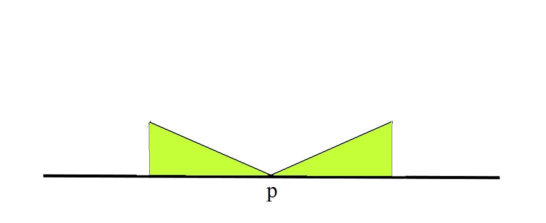
in the x-axis
with
. Each set
having Euclidean distance less than
from
, respectively.


 denotes the cardinality of the set
  is the minimum cardinality of a dense subset, i.e.,
  such that if
  . If
. If  .
. of
of  , there exists some
  such that
  . In other words, any non-empty open subset of
  , is the minimum cardinality of a network in the space
  .
. , is the minimum cardinality of a base for the space
  . If
. If  , then
  ,
,  has a countable network (see
  for any space
  does not hold, as indicated by the Sorgenfrey line. Monolithic spaces form a class of spaces in which the inequality
  holds for each space in the class and for each subspace of such a space.
  always holds. The inequality
  only holds for a restricted class of spaces. On the other hand, it is clear that
  for any space
  ,
,  . It is easy to verify that the following two statements are equivalent:
 . It is easy to verify that the following two statements are equivalent:
 -theory and the study of Corson compact spaces (see [1]).
 .
.  . Thus any space with a countable network is monolithic. However, any space that has a countable network but is not metrizable is not strongly monolithic, e.g., the function space
  direction, note that any compact metrizable space is separable (monolithicity is not needed). For the
  direction, note that any separable monolithic space has a countable network. Any compact space with a countable network is metrizable (see
 where
where  is the closed unit interval
  diagonal is metrizable (
 is metrizable.
 for a space
  is a point-countabe base if every point in
  such that
  is dense in
  be a one-point set to start with. For
  , let
, let  . Let
. Let  . For each finite
  such that
  , choose a point
  . Let
. Let  be the union of
  and the set of all points
  . Let
. Let  . Suppose we have
  . Let
. Let  . We know that
  is countable since every element of
  . We also know that
  . By the countably compactness of
  such that
  . The finite set
  must have appeared during the induction process of selecting points for
  (i.e.
(i.e.  (thus we have
  ). On the other hand, since
  , producing a contradiction. Thus the countable set
  of open covers of a space
  and each open set
  with
with  , there is some
  containing the point
  . A developable space is one that has a development. A Moore space is a regular developable space.
 of subsets of a space
  . An equivalent way of defining a development: A sequence
  is a local base at
  .
. always holds, we only need to show
  . To this end, we exhibit a base
  . Let
. Let  be a network with cardinality
  .
. , choose open set
  such that
  . Let
. Let  and
and  . Note that
  . Because
  is a cover of
  such that
  . There is some
  . Then
  . For each
  . The sequence
  works like a development. We have just shown that
  the weight (the least cardinality of a base for
  , we have
  . Now consider the case that
  is an uncountable cardinal. Based on the Bing-Nagata-Smirnov metrization theorem, any metrizable space has a
  discrete base. Let
  be a
be a  . Because each
  for each
  for some
  . If
. If  is the least upper bound of
  .
. . The idea is that we can obtain a base for
  (i.e.
(i.e.  , we only need to consider
  is compact, is a cover of the space
  , there is an open set
  and
and  is compact.
 for the open subspace
  .
. and
and  in Claim 1. Thus
  . Note that
  (the network weight of a subspace cannot exceed the original network weight). By the result in the previous post, we have
  . We now have
  (the weight of a subspace cannot exceed the weight of the space containing it). So the weight of any open subspace with compact closure cannot exceed
  .
. for any compact
  (Hausdorff and regular). Let
  for some
  where
where  where
where  .
. be the topology for the space
  . We can find a base
  that generates a weaker (coarser) topology such that
  . We can also find a base
  that generates a finer topology such that
  . These are restated as lemmas.
 on
on  .
. such that
  . Consider all pairs
  such that there exist disjoint
  with
with  and
and  . Such pairs exist because we are working in a Hausdorff space. Let
  and their finite interections. This is a base for a topology and let
  and this is a Hausdorff topology. Note that
  .
. on
on  .
. . It is also clear that
  always holds. For compact spaces, we have
  .
. denote
  be a continuous function mapping a separable metric space
  is a network for
  . It follows that
  set (thus every closed set is a
  where
where and
and .
. is of the form
  where
where  and all points
  having distance
  from
from  and
and  coincide with the usual topology on
  spaces, J. Math. Mech. 15, 983-1002.
 is not normal.
 and for each
  , there is some
  such that
  . The network weight of
  and
and  as follows. It can be shown that these two closed subsets of

 and
and  are open subsets of
  and
and  . It is shown below that
  .
. be the set of all irrational numbers and let
  be the set of all rational numbers. For each
  , choose some real number
  such that
 . Obviously
  . Since
  subset of
  , there exists
  and there exists an
  such that
  is in the closure of
  in the usual topology of
  is in the closure of
  , the open set
  would have to contain points of
  be an open set containing the point
  is of the form
 . Since
  such that
  . It does not matter whether the point
  must overlap with the interval
  . Then pick
  must overlap with the interval
  . Then pick
  belongs to the open set

 as defined above. The open set
  , establishing that the point