Bing’s Example G is an example of a topological space that is normal but not collectionwise normal. It was introduced in an influential paper of R. H. Bing in 1951 (see [1]). This paper has a metrization theorem that is now called Bing’s metrization theorem (any regular space is metrizable if and only if it has a  -discrete base). The paper also introduced the notion of collectionwise normality and discussed the roles it plays in metrization theory (e.g. a Moore space is metrizable if and only if it is collectionwise normal). Example G was an influential example from an influential paper. It became the basis of construction for many other counterexamples (see [5] for one example). Investigations were also conducted by looking at various covering properties among subspaces of Example G (see [2] and [4] are two examples).
In this post we prove some basic results about Bing’s Example G. Some of the results we prove are found in Bing’s 1951 paper. The other results shown here are usually mentioned without proof in various places in the literature.
____________________________________________________________________
Bing’s Example G – Definition
Let  be any uncountable set. Let
  be the set of all subsets of . Let
  be the set of all functions
  . Another notation for
  is the Cartesian product
  . For each
  , define the function
  by the following:
Let  . Let
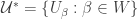
. Let  be the set of all open subsets of in the product topology. We now consider another topology on generated by the following base:
Bing’s Example G is the set with the topology generated by the base  . In other words, each
  is made an isolated point and points in
  retain the usual product open sets.
____________________________________________________________________
Bing’s Example G – Initial Discussion
Bing’s Example G, i.e. the space  as defined above, is obtained by altering the topology of the product space of
  many copies of the two-point discrete space where
  is the cardinality of the power set of the uncountable index set we start with. Out of this product space, a set of points is carefully chosen such that has the same cardinality as and such that is relatively discrete in the product space. Points in are made to retain the product topology and all points outside of are declared as isolated points.
We now show that the set is a discrete set in the space . For each , let  be the open set defined by
 .
.
It is clear that  is the only point of belonging to . Therefore, in the Example G topology, the set is discrete and closed . In the section “Bing’s Example G is not Collectionwise Hausdorff” below, we show below that cannot be separated by any pairwise disjoint collection of open sets.
The character at a point is the minimum cardinality of a local base at that point. The character at a point in in the Example G topology agrees with the product topology. Points in have character  . Specifically if the starting has cardinality
  , then points in have character
  . Thus Example G has large character and cannot be a Moore space (any Moore space has a countable base at every point).
____________________________________________________________________
Bing’s Example G is Normal
Let  and
and  be disjoint closed subsets of . The easy case is that one of and is a subset of
  , say
, say  . Then is a closed and open set in . Then and
  are disjoint open sets containing and , respectively. So we can assume that both
  and
and  .
.
Let  and
and  . Let
. Let 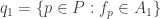 and
and 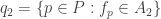 . Define the following open sets:
Because  , we have
  and
and  . Furthermore,
  . Let
. Let 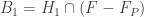 and
and 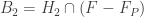 , which are open since they consist of isolated points. Then
  and
and  are disjoint open subsets of with
  and
and  .
.
____________________________________________________________________
Collectionwise Normal Spaces
Let  be a space. Let
  be a collection of subsets of . We say is pairwise disjoint if
  whenever
  with
with  . We say is discrete if for each
  , there is an open set
  containing
  such that intersects at most one set in .
The space is said to be collectionwise normal if for every discrete collection  of closed subsets fo , there is a pairwise disjoint collection
  of open subsets of such that
  for each
  . Every paracompact space is collectionwise normal (see Theorem 5.1.18, p.305 of [3]). Thus Bing’s Example G is not paracompact.
When discrete collection of closed sets in the definition of “collectionwise normal” is replaced by discrete collection of singleton sets, the space is said to be collectionwise Hausdorff. Clearly any collectionwise normal space is collectionwise Hausdorff. Bing’s Example is actually not collectionwise Hausdorff.
____________________________________________________________________
Bing’s Example G is not Collectionwise Hausdorff
The discrete set cannot be separated by disjoint open sets. For each , let  be an open subset of such that
  . We show that the open sets cannot be pairwise disjoint. For each , choose an open set
  in the product topology of such that
  . The product space is a product of separable spaces, hence has the countable chain condition (CCC). Thus the open sets cannot be pairwise disjoint. Thus
  and
and  for at least two points
  .
.
____________________________________________________________________
Bing’s Example G is Completely Normal
The proof for showing Bing’s Example G is normal can be modified to show that it is completely normal. First some definitions. Let be a space. Let  and
and  . The sets
  and
and  are separated sets if
  . Essentially, any two disjoint sets are separated sets if and only if none of them contains limit points (i.e. accumulation points) of the other set. A space is said to be completely normal if for every two separated sets and in , there exist disjoint open subsets
  and
and  of such that
  and
and  . Any two disjoint closed sets are separated sets. Thus any completely normal space is normal. It is well known that for any regular space , is completely normal if and only if is hereditarily normal. For more about completely normality, see [3] and [6].
Let  and
and  such that
  . We consider two cases. One is that one of and is a subset of . The other is that both and .
The first case. Suppose . Then consists of isolated points and is an open subset of . For each  , choose an open subset
  of such that
  and contains no points of
  and
and  . For each
  , let
, let  . Let be the union of all where
  . Let
. Let  . Then and are disjoint open sets with
  and
and  .
.
The second case. Suppose  and
and  . Let and . Define the following open sets:
Because , we have and . Furthermore, . Let and , which are open since they consist of isolated points. Then  and
and  are disjoint open subsets of with and .
____________________________________________________________________
Bing’s Example G is not Perfectly Normal
A space is perfectly normal if it is normal and that every closed subset is  (i.e. the intersection of countably many open subsets). The set of non-isolated points is a closed set in . We show that cannot be a -set. Before we do so, we need to appeal to a fact about the product space .
According to the Tychonoff theorem, the product space is a compact space since it is a product of compact spaces. On the other hand, is a product of uncountably many factors and is thus not first countable. It is a well known fact that in a compact Hausdorff space, if a point is a -point, then there is a countable local base at that point (i.e. the space is first countable at that point). Thus no point of the compact product space can be a -point. Since points of retain the open sets of the product topology, no point of can be a -point in the Bing’s Example G topology.
For each , let be open in such that  and contains no points
  . For example, we can define as in the above section “Bing’s Example G – Initial Discussion”.
Suppose that is a -set. Then  where each
  is an open subset of . Now for each , we have
  , contradicting the fact that the point cannot be a -point in the space (and in the product space ). Thus is not a -set in the space , leading to the conclusion that Bing’s Example G is not perfectly normal.
____________________________________________________________________
Bing’s Example G is not Metacompact
A space  is said to have caliber if for every uncountable collection
  of non-empty open subsets of , there is an uncountable
  such that
  . Any product of separable spaces has this property (see Topological Spaces with Caliber Omega 1). Thus the product space has caliber . Thus in the product space , no collection of uncountably many non-empty open sets can be a point-finite collection (in fact cannot even be point-countable).
To see that the Example G is not metacompact, let  be a collection of open sets such that for , , is open in the product topology of and contains no points . For example, we can define as in the above section “Bing’s Example G – Initial Discussion”.
Let  . Let
. Let  . Any open refinement of
  would contain uncountably many open sets in the product topology and thus cannot be point-finite. Thus the space cannot be metacompact.
____________________________________________________________________
Reference
- Bing, R. H., Metrization of Topological Spaces, Canad. J. Math., 3, 175-186, 1951.
- Burke, D. K., A note on R. H. Bing’s example G, Top. Conf. VPI, Lectures Notes in Mathematics, 375, Springer Verlag, New York, 47-52, 1974.
- Engelking, R., General Topology, Revised and Completed edition, Heldermann Verlag, Berlin, 1989.
- Lewis, I. W., On covering properties of subspaces of R. H. Bing’s Example G, Gen. Topology Appl., 7, 109-122, 1977.
- Michael, E., Point-finite and locally finite coverings, Canad. J. Math., 7, 275-279, 1955.
- Willard, S., General Topology, Addison-Wesley Publishing Company, 1970.
____________________________________________________________________

 ,
,  if
if  and
and  if
if 


 .
.

 (for any uncountable cardinal
  -system) if there is a set
  such that for every
  with
with  . When such set
  such that
  is a family of spaces such that
  has caliber
  . Then
  has caliber
  where
where  for all but finitely many
  . Let
. Let  be an uncountable collection of such non-empty open sets. Our plan is to find an uncountable
  such that
  .
.
 , let
, let  be the finite set such that
  if and only if
  . Consider
  . By the Delta-system lemma, there is an uncountable
  such that
  is a Delta-system. Let
  and
and  where
where  , we have
  . For each
  , we have
  in
in  . Then we can define an
  in
in  and we have
  .
. . For each
  where
where  be
be  (i.e.
(i.e.  is a projection map). Let
 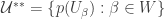 .
. is countable. The second is that
  such that
  for all
  . Then fix
  and choose
  . Then
  is extendable to some
  in
in  for all
  . Thus we have
 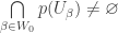 . Choose
  . As in the previous case,
 where
where  of the product space
  (
( such that
  for at most countably many
  . Note that
  is a space with the CCC since it is a product of separable spaces. Furthermore
  where each
  . Note that each
  belongs to at most countably many
  . Thus for any uncountable
  .
. with a topology finer than the usual topology obtained by isolating each point in
  where
where  to denote this topological space. It is a classic result that
  is not normal (see
  is paracompact and perfectly normal. We also use this result to show that if
  is a separable metric space, then
  of
of  -subset of a paracompact space is paracompact.
 be a paracompact space. Let
  be a dense Lindelof subspace. Let
  refines
  be a locally finite open refinement of
  such that it is a cover of
  ,
,  .
. come from a locally finite collection, they are closure preserving. Hence we have:
 , choose some
  such that
  . Then
  is a countable subcollection of
  Suppose
  be an non-empty open set. For each
  , let
, let  (the space is assumed to be regular). By assumption, the open set
  .
.  Suppose
  where each
  is a closed set in
  , then
  . Let
. Let  be a base for
  is locally finite in
  such that we can choose nonempty open set
  with
with  . Since
  exist. Let
  be the collection of all non-empty
  . For each
  . Of course, each
  is still locally finite.
 is closed in
  and each
  , consider the following collection:
 is a closed set in
  . The set
  is a union of closed sets. In general, the union of closed sets needs not be closed. However,

 , which is the union of countably many closed sets.
  where
where 

 . Each
  is an open cover of
  be a locally finite open refinement of

 is a locally finite collection. The open cover
  is Lindelof. Furthermore
  (in words every point of the space belongs to one set in the collection). Furthermore,
  such that
  . The cover
  and
and  of
of  such that each
  is a locally finite collection of subsets of
  of
of  such that
  for each
  .
.
 such that
  where each
  is a closed subset of
  , let
, let  be open in
  .
.  be the set of all
  . Let
. Let  be a locally finite refinement of
  . Let
. Let  be the following:
 is a
is a  such that
  , there is an open set
  such that
 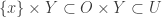 .
. such that
  is a cover of
  . By the Tube Lemma, for each
  such that
  . Since
  be a locally finite open refinement of
  such that
  for each
  . We claim that
  . Then
  for some
  and
and  . Thus,
 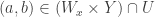 for some
  . Secondly, it is clear that
  . Then
  can meet only finitely many sets in
  . For example, we can let
  , which is the Stone-Cech compactification of
  is paracompact. Note that
  and each
  is a closed subset of
  ).
). of rational numbers. The same proof that
  is not normal.
 . The set
  and
and  . The set
  that is of first category in the real line,
  is at most countable. The Russian mathematician Luzin in 1914 constructed such an uncountable Luzin set using continuum hypothesis (CH). A good reference for Luzin sets is [4]. We have the following theorem.
 be the set of all closed nowhere dense sets in the real line. Choose a real number
  to start. For each
  with
with  , choose a real number
  not in the following set:
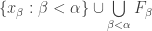
 . Then
  is a Luzin set.
  contains all but countably many points of
  are closed nowhere dense subsets of the real line, then
  contains all but countably many points of the Luzin set
  be uncountable and dense in the real line such that
  is uncountable. Given a dense
  can only contain countably many points of
  where each
  be open in the real line such that
  . Each
  contains all but countably many points of the Luzin set
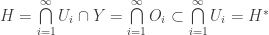
 . Then
  cannot be an
  be a countable dense subset of the real line. The set
  ,
,  . It is clear that adding countably many points to a Luzin set still results in a Luzin set. Thus
  are discrete and points in
  is dense in the real line.