Bing’s Example G

Posted on November 18, 2012 by Dan Ma

Bing’s Example G is an example of a topological space that is normal but not collectionwise normal. It was introduced in an influential paper of R. H. Bing in 1951 (see [1]). This paper has a metrization theorem that is now called Bing’s metrization theorem (any regular space is metrizable if and only if it has a $\sigma$ -discrete base). The paper also introduced the notion of collectionwise normality and discussed the roles it plays in metrization theory (e.g. a Moore space is metrizable if and only if it is collectionwise normal). Example G was an influential example from an influential paper. It became the basis of construction for many other counterexamples (see [5] for one example). Investigations were also conducted by looking at various covering properties among subspaces of Example G (see [2] and [4] are two examples).

In this post we prove some basic results about Bing’s Example G. Some of the results we prove are found in Bing’s 1951 paper. The other results shown here are usually mentioned without proof in various places in the literature.

____________________________________________________________________

Bing’s Example G – Definition

Let $P$ be any uncountable set. Let $Q$ be the set of all subsets of $P$ . Let $F=2^Q$ be the set of all functions $f: Q \rightarrow 2=\left\{0,1 \right\}$ . Another notation for $2^Q$ is the Cartesian product $\prod \limits_{q \in Q} \left\{0,1 \right\}$ . For each $p \in P$ , define the function $f_p: Q \rightarrow 2$ by the following:

$\forall q \in Q$

$f_p(q)=1$

$p \in q$

$f_p(q)=0$

$p \notin q$

Let $F_P=\left\{f_p: p \in P \right\}$ . Let $\tau$ be the set of all open subsets of $2^Q$ in the product topology. We now consider another topology on $2^Q$ generated by the following base:

$\mathcal{B}=\tau \cup \left\{\left\{x \right\}: x \in F-F_P \right\}$

Bing’s Example G is the set $F=2^Q$ with the topology generated by the base $\mathcal{B}$ . In other words, each $x \in F-F_P$ is made an isolated point and points in $F_P$ retain the usual product open sets.

____________________________________________________________________

Bing’s Example G – Initial Discussion

Bing’s Example G, i.e. the space $F$ as defined above, is obtained by altering the topology of the product space of $2^{\lvert \mathcal{K} \lvert}$ many copies of the two-point discrete space where $\mathcal{K}$ is the cardinality of the power set of the uncountable index set $P$ we start with. Out of this product space, a set $F_P$ of points is carefully chosen such that $F_P$ has the same cardinality as $P$ and such that $F_P$ is relatively discrete in the product space. Points in $F_P$ are made to retain the product topology and all points outside of $F_P$ are declared as isolated points.

We now show that the set $F_P$ is a discrete set in the space $F$ . For each $p \in P$ , let $W_p$ be the open set defined by

$W_p=\left\{f \in F: f(\left\{p \right\})=1 \text{ and } f(P-\left\{p \right\})=0 \right\}$ .

It is clear that $f_p$ is the only point of $F_P$ belonging to $W_p$ . Therefore, in the Example G topology, the set $F_P$ is discrete and closed . In the section “Bing’s Example G is not Collectionwise Hausdorff” below, we show below that $F_P$ cannot be separated by any pairwise disjoint collection of open sets.

The character at a point is the minimum cardinality of a local base at that point. The character at a point in $F_P$ in the Example G topology agrees with the product topology. Points in $F_P$ have character $\lvert Q \lvert=2^{\lvert P \lvert}$ . Specifically if the starting $P$ has cardinality $\omega_1$ , then points in $F_P$ have character $2^{\omega_1}$ . Thus Example G has large character and cannot be a Moore space (any Moore space has a countable base at every point).

____________________________________________________________________

Bing’s Example G is Normal

Let $H_1$ and $H_2$ be disjoint closed subsets of $F$ . The easy case is that one of $H_1$ and $H_2$ is a subset of $F-F_P$ , say $H_1 \subset F-F_P$ . Then $H_1$ is a closed and open set in $F$ . Then $H_1$ and $F-H_1$ are disjoint open sets containing $H_1$ and $H_2$ , respectively. So we can assume that both $H_1 \cap F_P \ne \varnothing$ and $H_2 \cap F_P \ne \varnothing$ .

Let $A_1=H_1 \cap F_P$ and $A_2=H_2 \cap F_P$ . Let $q_1=\left\{p \in P: f_p \in A_1 \right\}$ and $q_2=\left\{p \in P: f_p \in A_2 \right\}$ . Define the following open sets:

$U_1=\left\{f \in F: f(q_1)=1 \text{ and } f(q_2)=0 \right\}$

$U_2=\left\{f \in F: f(q_1)=0 \text{ and } f(q_2)=1 \right\}$

Because $H_1 \cap H_2=\varnothing$ , we have $A_1 \subset U_1$ and $A_2 \subset U_2$ . Furthermore, $U_1 \cap U_2=\varnothing$ . Let $B_1=H_1 \cap (F-F_P)$ and $B_2=H_2 \cap (F-F_P)$ , which are open since they consist of isolated points. Then $O_1=(U_1 \cup B_1)-H_2$ and $O_2=(U_2 \cup B_2)-H_1$ are disjoint open subsets of $F$ with $H_1 \subset O_1$ and $H_2 \subset O_2$ .

____________________________________________________________________

Collectionwise Normal Spaces

Let $X$ be a space. Let $\mathcal{A}$ be a collection of subsets of $X$ . We say $\mathcal{A}$ is pairwise disjoint if $A \cap B=\varnothing$ whenever $A,B \in \mathcal{A}$ with $A \ne B$ . We say $\mathcal{A}$ is discrete if for each $x \in X$ , there is an open set $O$ containing $x$ such that $O$ intersects at most one set in $\mathcal{A}$ .

The space $X$ is said to be collectionwise normal if for every discrete collection $\mathcal{D}$ of closed subsets fo $X$ , there is a pairwise disjoint collection $\left\{U_D: D \in \mathcal{D} \right\}$ of open subsets of $X$ such that $D \subset U_D$ for each $D \in \mathcal{D}$ . Every paracompact space is collectionwise normal (see Theorem 5.1.18, p.305 of [3]). Thus Bing’s Example G is not paracompact.

When discrete collection of closed sets in the definition of “collectionwise normal” is replaced by discrete collection of singleton sets, the space is said to be collectionwise Hausdorff. Clearly any collectionwise normal space is collectionwise Hausdorff. Bing’s Example is actually not collectionwise Hausdorff.

____________________________________________________________________

Bing’s Example G is not Collectionwise Hausdorff

The discrete set $F_P$ cannot be separated by disjoint open sets. For each $p \in P$ , let $O_p$ be an open subset of $F$ such that $p \in O_p$ . We show that the open sets $O_p$ cannot be pairwise disjoint. For each $p \in P$ , choose an open set $L_p$ in the product topology of $2^Q$ such that $p \in L_p \subset O_p$ . The product space $2^Q$ is a product of separable spaces, hence has the countable chain condition (CCC). Thus the open sets $L_p$ cannot be pairwise disjoint. Thus $L_t \cap L_s \ne \varnothing$ and $O_t \cap O_s \ne \varnothing$ for at least two points $s,t \in P$ .

____________________________________________________________________

Bing’s Example G is Completely Normal

The proof for showing Bing’s Example G is normal can be modified to show that it is completely normal. First some definitions. Let $X$ be a space. Let $A \subset X$ and $B \subset X$ . The sets $A$ and $B$ are separated sets if $A \cap \overline{B}=\varnothing=\overline{A} \cap B$ . Essentially, any two disjoint sets are separated sets if and only if none of them contains limit points (i.e. accumulation points) of the other set. A space $X$ is said to be completely normal if for every two separated sets $A$ and $B$ in $X$ , there exist disjoint open subsets $U$ and $V$ of $X$ such that $A \subset U$ and $B \subset V$ . Any two disjoint closed sets are separated sets. Thus any completely normal space is normal. It is well known that for any regular space $X$ , $X$ is completely normal if and only if $X$ is hereditarily normal. For more about completely normality, see [3] and [6].

Let $H_1 \subset F$ and $H_2 \subset F$ such that $H_1 \cap \overline{H_2}=\varnothing=\overline{H_1} \cap H_2$ . We consider two cases. One is that one of $H_1$ and $H_2$ is a subset of $F-F_P$ . The other is that both $H_1 \cap F_P \ne \varnothing$ and $H_2 \cap F_P \ne \varnothing$ .

The first case. Suppose $H_1 \subset F-F_P$ . Then $H_1$ consists of isolated points and is an open subset of $F$ . For each $x \in H_2 \cap F_P$ , choose an open subset $V_x$ of $F$ such that $x \in V_x$ and $V_x$ contains no points of $F_P-\left\{ x \right\}$ and $V_x \cap \overline{H_1}=\varnothing$ . For each $x \in H_2 \cap (F-F_P)$ , let $V_x=\left\{x \right\}$ . Let $V$ be the union of all $V_x$ where $x \in H_2$ . Let $U=H_1$ . Then $U$ and $V$ are disjoint open sets with $H_1 \subset U$ and $H_2 \subset V$ .

The second case. Suppose $A_1=H_1 \cap F_P \ne \varnothing$ and $A_2=H_2 \cap F_P \ne \varnothing$ . Let $q_1=\left\{p \in P: f_p \in A_1 \right\}$ and $q_2=\left\{p \in P: f_p \in A_2 \right\}$ . Define the following open sets:

$U_1=\left\{f \in F: f(q_1)=1 \text{ and } f(q_2)=0 \right\}$

$U_2=\left\{f \in F: f(q_1)=0 \text{ and } f(q_2)=1 \right\}$

Because $H_1 \cap H_2=\varnothing$ , we have $A_1 \subset U_1$ and $A_2 \subset U_2$ . Furthermore, $U_1 \cap U_2=\varnothing$ . Let $B_1=H_1 \cap (F-F_P)$ and $B_2=H_2 \cap (F-F_P)$ , which are open since they consist of isolated points. Then $O_1=(U_1 \cup B_1)-\overline{H_2}$ and $O_2=(U_2 \cup B_2)-\overline{H_1}$ are disjoint open subsets of $F$ with $H_1 \subset O_1$ and $H_2 \subset O_2$ .

____________________________________________________________________

Bing’s Example G is not Perfectly Normal

A space is perfectly normal if it is normal and that every closed subset is $G_\delta$ (i.e. the intersection of countably many open subsets). The set $F_P$ of non-isolated points is a closed set in $F$ . We show that $F_P$ cannot be a $G_\delta$ -set. Before we do so, we need to appeal to a fact about the product space $2^Q$ .

According to the Tychonoff theorem, the product space $2^Q$ is a compact space since it is a product of compact spaces. On the other hand, $2^Q$ is a product of uncountably many factors and is thus not first countable. It is a well known fact that in a compact Hausdorff space, if a point is a $G_\delta$ -point, then there is a countable local base at that point (i.e. the space is first countable at that point). Thus no point of the compact product space $2^Q$ can be a $G_\delta$ -point. Since points of $F_P$ retain the open sets of the product topology, no point of $F_P$ can be a $G_\delta$ -point in the Bing’s Example G topology.

For each $p \in P$ , let $W_p$ be open in $F$ such that $f_p \in W_p$ and $W_p$ contains no points $F_P-\left\{f_p \right\}$ . For example, we can define $W_p$ as in the above section “Bing’s Example G – Initial Discussion”.

Suppose that $F_P$ is a $G_\delta$ -set. Then $F_P=\bigcap \limits_{i=1}^\infty O_i$ where each $O_i$ is an open subset of $F$ . Now for each $p \in P$ , we have $\left\{f_p \right\}=\bigcap \limits_{i=1}^\infty (O_i \cap W_p)$ , contradicting the fact that the point $f_p$ cannot be a $G_\delta$ -point in the space $F$ (and in the product space $2^Q$ ). Thus $F_P$ is not a $G_\delta$ -set in the space $F$ , leading to the conclusion that Bing’s Example G is not perfectly normal.

____________________________________________________________________

Bing’s Example G is not Metacompact

A space $M$ is said to have caliber $\omega_1$ if for every uncountable collection $\left\{U_\alpha: \alpha < \omega_1 \right\}$ of non-empty open subsets of $M$ , there is an uncountable $A \subset \omega_1$ such that $\bigcap \left\{U_\alpha: \alpha \in A \right\} \ne \varnothing$ . Any product of separable spaces has this property (see Topological Spaces with Caliber Omega 1). Thus the product space $2^Q$ has caliber $\omega_1$ . Thus in the product space $2^Q$ , no collection of uncountably many non-empty open sets can be a point-finite collection (in fact cannot even be point-countable).

To see that the Example G is not metacompact, let $\mathcal{W}=\left\{W_p: p \in P \right\}$ be a collection of open sets such that for $p \in P$ , $f_p \in W_p$ , $W_p$ is open in the product topology of $2^Q$ and $W_p$ contains no points $F_P-\left\{f_p \right\}$ . For example, we can define $W_p$ as in the above section “Bing’s Example G – Initial Discussion”.

Let $W=\bigcup \mathcal{W}$ . Let $\mathcal{V}=\mathcal{W} \cup \left\{\left\{ x \right\}: x \in F-W \right\}$ . Any open refinement of $\mathcal{V}$ would contain uncountably many open sets in the product topology and thus cannot be point-finite. Thus the space $F$ cannot be metacompact.

____________________________________________________________________

Reference

Bing, R. H., Metrization of Topological Spaces, Canad. J. Math., 3, 175-186, 1951.
Burke, D. K., A note on R. H. Bing’s example G, Top. Conf. VPI, Lectures Notes in Mathematics, 375, Springer Verlag, New York, 47-52, 1974.
Engelking, R., General Topology, Revised and Completed edition, Heldermann Verlag, Berlin, 1989.
Lewis, I. W., On covering properties of subspaces of R. H. Bing’s Example G, Gen. Topology Appl., 7, 109-122, 1977.
Michael, E., Point-finite and locally finite coverings, Canad. J. Math., 7, 275-279, 1955.
Willard, S., General Topology, Addison-Wesley Publishing Company, 1970.

____________________________________________________________________

$\copyright \ \ 2012$

Michael Line Basics

Posted on October 28, 2012 by Dan Ma

Like the Sorgenfrey line, the Michael line is a classic counterexample that is covered in standard topology textbooks and in first year topology courses. This easily accessible example helps transition students from the familiar setting of the Euclidean topology on the real line to more abstract topological spaces. One of the most famous results regarding the Michael line is that the product of the Michael line with the space of the irrational numbers is not normal. Thus it is an important example in demonstrating the pathology in products of paracompact spaces. The product of two paracompact spaces does not even have be to be normal, even when one of the factors is a complete metric space. In this post, we discuss this classical result and various other basic results of the Michael line.

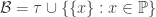
Let $\mathbb{R}$ be the real number line. Let $\mathbb{P}$ be the set of all irrational numbers. Let $\mathbb{Q}=\mathbb{R}-\mathbb{P}$ , the set of all rational numbers. Let $\tau$ be the usual topology of the real line $\mathbb{R}$ . The following is a base that defines a topology on $\mathbb{R}$ .

$\mathcal{B}=\tau \cup \left\{\left\{ x \right\}: x \in \mathbb{P}\right\}$

The real line with the topology generated by $\mathcal{B}$ is called the Michael line and is denoted by $\mathbb{M}$ . In essense, in $\mathbb{M}$ , points in $\mathbb{P}$ are made isolated and points in $\mathbb{Q}$ retain the usual Euclidean open sets.

The Euclidean topology $\tau$ is coarser (weaker) than the Michael line topology (i.e. $\tau$ being a subset of the Michael line topology). Thus the Michael line is Hausdorff. Since the Michael line topology contains a metrizable topology, $\mathbb{M}$ is submetrizable (submetrized by the Euclidean topology). It is clear that $\mathbb{M}$ is first countable. Having uncountably many isolated points, the Michael line does not have the countable chain condition (thus is not separable). The following points are discussed in more details.

The space $\mathbb{M}$ is paracompact.
The space $\mathbb{M}$ is not Lindelof.
The extent of the space $\mathbb{M}$ is $c$ where $c$ is the cardinality of the real line.
The space $\mathbb{M}$ is not locally compact.
The space $\mathbb{M}$ is not perfectly normal, thus not metrizable.
The space $\mathbb{M}$ is not a Moore space, but has a $G_\delta$ -diagonal.
The product $\mathbb{M} \times \mathbb{P}$ is not normal where $\mathbb{P}$ has the usual topology.
The product $\mathbb{M} \times \mathbb{P}$ is metacompact.
The space $\mathbb{M}$ has a point-countable base.
For each $n=1,2,3,\cdots$ , the product $\mathbb{M}^n$ is paracompact.

Finite and Countable Products of the Michael Line

The product $\mathbb{M}^\omega$ is not normal.

Finite and Countable Products of the Michael Line

There exist a Lindelof space $L$ and a separable metric space $W$ such that $L \times W$ is not normal.

Bernstein Sets and the Michael Line

Results 10, 11 and 12 are shown in some subsequent posts.

___________________________________________________________________________________

Baire Category Theorem

Before discussing the Michael line in greater details, we point out one connection between the Michael line topology and the Euclidean topology on the real line. The Michael line topology on $\mathbb{Q}$ coincides with the Euclidean topology on $\mathbb{Q}$ . A set is said to be a $G_\delta$ -set if it is the intersection of countably many open sets. By the Baire category theorem, the set $\mathbb{Q}$ is not a $G_\delta$ -set in the Euclidean real line (see the section called “Discussion of the Above Question” in the post A Question About The Rational Numbers). Thus the set $\mathbb{Q}$ is not a $G_\delta$ -set in the Michael line. This fact is used in Result 5.

The fact that $\mathbb{Q}$ is not a $G_\delta$ -set in the Euclidean real line implies that $\mathbb{P}$ is not an $F_\sigma$ -set in the Euclidean real line. This fact is used in Result 7.

___________________________________________________________________________________

Result 1

Let $\mathcal{U}$ be an open cover of $\mathbb{M}$ . We proceed to derive a locally finite open refinement $\mathcal{V}$ of $\mathcal{U}$ . Recall that $\tau$ is the usual topology on $\mathbb{R}$ . Assume that $\mathcal{U}$ consists of open sets in the base $\mathcal{B}$ . Let $\mathcal{U}_\tau=\mathcal{U} \cap \tau$ . Let $Y=\cup \mathcal{U}_\tau$ . Note that $Y$ is a Euclidean open subspace of the real line (hence it is paracompact). Then there is $\mathcal{V}_\tau \subset \tau$ such that $\mathcal{V}_\tau$ is a locally finite open refinement $\mathcal{V}_\tau$ of $\mathcal{U}_\tau$ and such that $\mathcal{V}_\tau$ covers $Y$ (locally finite in the Euclidean sense). Then add to $\mathcal{V}_\tau$ all singleton sets $\left\{ x \right\}$ where $x \in \mathbb{M}-Y$ and let $\mathcal{V}$ denote the resulting open collection.

The resulting $\mathcal{V}$ is a locally finite open collection in the Michael line $\mathbb{M}$ . Furthermore, $\mathcal{V}$ is also a refinement of the original open cover $\mathcal{U}$ . $\blacksquare$

A similar argument shows that $\mathbb{M}$ is hereditarily paracompact.

___________________________________________________________________________________

Result 2

To see that $\mathbb{M}$ is not Lindelof, observe that there exist Euclidean uncountable closed sets consisting entirely of irrational numbers (i.e. points in $\mathbb{P}$ ). For example, it is possible to construct a Cantor set entirely within $\mathbb{P}$ .

Let $C$ be an uncountable Euclidean closed set consisting entirely of irrational numbers. Then this set $C$ is an uncountable closed and discrete set in $\mathbb{M}$ . In any Lindelof space, there exists no uncountable closed and discrete subset. Thus the Michael line $\mathbb{M}$ cannot be Lindelof. $\blacksquare$

___________________________________________________________________________________

Result 3

The argument in Result 2 indicates a more general result. First, a brief discussion of the cardinal function extent. The extent of a space $X$ is the smallest infinite cardinal number $\mathcal{K}$ such that every closed and discrete set in $X$ has cardinality $\le \mathcal{K}$ . The extent of the space $X$ is denoted by $e(X)$ . When the cardinal number $e(X)$ is $e(X)=\aleph_0$ (the first infinite cardinal number), the space $X$ is said to have countable extent, meaning that in this space any closed and discrete set must be countably infinite or finite. When $e(X)>\aleph_0$ , there are uncountable closed and discrete subsets in the space.

It is straightforward to see that if a space $X$ is Lindelof, the extent is $e(X)=\aleph_0$ . However, the converse is not true.

The argument in Result 2 exhibits a closed and discrete subset of $\mathbb{M}$ of cardinality $c$ . Thus we have $e(\mathbb{M})=c$ . $\blacksquare$

___________________________________________________________________________________

Result 4

The Michael line $\mathbb{M}$ is not locally compact at all rational numbers. Observe that the Michael line closure of any Euclidean open interval is not compact in $\mathbb{M}$ . $\blacksquare$

___________________________________________________________________________________

Result 5

A set is said to be a $G_\delta$ -set if it is the intersection of countably many open sets. A space is perfectly normal if it is a normal space with the additional property that every closed set is a $G_\delta$ -set. In the Michael line $\mathbb{M}$ , the set $\mathbb{Q}$ of rational numbers is a closed set. Yet, $\mathbb{Q}$ is not a $G_\delta$ -set in the Michael line (see the discussion above on the Baire category theorem). Thus $\mathbb{M}$ is not perfectly normal and hence not a metrizable space. $\blacksquare$

___________________________________________________________________________________

Result 6

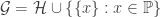
The diagonal of a space $X$ is the subset of its square $X \times X$ that is defined by $\Delta=\left\{(x,x): x \in X \right\}$ . If the space is Hausdorff, the diagonal is always a closed set in the square. If $\Delta$ is a $G_\delta$ -set in $X \times X$ , the space $X$ is said to have a $G_\delta$ -diagonal. It is well known that any metric space has $G_\delta$ -diagonal. Since $\mathbb{M}$ is submetrizable (submetrized by the usual topology of the real line), it has a $G_\delta$ -diagonal too.

Any Moore space has a $G_\delta$ -diagonal. However, the Michael line is an example of a space with $G_\delta$ -diagonal but is not a Moore space. Paracompact Moore spaces are metrizable. Thus $\mathbb{M}$ is not a Moore space. For a more detailed discussion about Moore spaces, see Sorgenfrey Line is not a Moore Space. $\blacksquare$

___________________________________________________________________________________

Result 7

We now show that $\mathbb{M} \times \mathbb{P}$ is not normal where $\mathbb{P}$ has the usual topology. In this proof, the following two facts are crucial:

The set $\mathbb{P}$ is not an $F_\sigma$ -set in the real line.
The set $\mathbb{P}$ is dense in the real line.

Let $H$ and $K$ be defined by the following:

$H=\left\{(x,x): x \in \mathbb{P} \right\}$

$K=\mathbb{Q} \times \mathbb{P}$

The sets $H$ and $K$ are disjoint closed sets in $\mathbb{M} \times \mathbb{P}$ . We show that they cannot be separated by disjoint open sets. To this end, let $H \subset U$ and $K \subset V$ where $U$ and $V$ are open sets in $\mathbb{M} \times \mathbb{P}$ .

To make the notation easier, for the remainder of the proof of Result 7, by an open interval $(a,b)$ , we mean the set of all real numbers $t$ with $a<t<b$ . By $(a,b)^*$ , we mean $(a,b) \cap \mathbb{P}$ . For each $x \in \mathbb{P}$ , choose an open interval $U_x=(a,b)^*$ such that $\left\{x \right\} \times U_x \subset U$ . We also assume that $x$ is the midpoint of the open interval $U_x$ . For each positive integer $k$ , let $P_k$ be defined by:

$P_k=\left\{x \in \mathbb{P}: \text{ length of } U_x > \frac{1}{k} \right\}$

Note that $\mathbb{P}=\bigcup \limits_{k=1}^\infty P_k$ . For each $k$ , let $T_k=\overline{P_k}$ (Euclidean closure in the real line). It is clear that $\bigcup \limits_{k=1}^\infty P_k \subset \bigcup \limits_{k=1}^\infty T_k$ . On the other hand, $\bigcup \limits_{k=1}^\infty T_k \not\subset \bigcup \limits_{k=1}^\infty P_k=\mathbb{P}$ (otherwise $\mathbb{P}$ would be an $F_\sigma$ -set in the real line). So there exists $T_n=\overline{P_n}$ such that $\overline{P_n} \not\subset \mathbb{P}$ . So choose a rational number $r$ such that $r \in \overline{P_n}$ .

Choose a positive integer $j$ such that $\frac{2}{j}<\frac{1}{n}$ . Since $\mathbb{P}$ is dense in the real line, choose $y \in \mathbb{P}$ such that $r-\frac{1}{j}<y<r+\frac{1}{j}$ . Now we have $(r,y) \in K \subset V$ . Choose another integer $m$ such that $\frac{1}{m}<\frac{1}{j}$ and $(r-\frac{1}{m},r+\frac{1}{m}) \times (y-\frac{1}{m},y+\frac{1}{m})^* \subset V$ .

Since $r \in \overline{P_n}$ , choose $x \in \mathbb{P}$ such that $r-\frac{1}{m}<x<r+\frac{1}{m}$ . Now it is clear that $(x,y) \in V$ . The following inequalities show that $(x,y) \in U$ .

$\lvert x-y \lvert \le \lvert x-r \lvert + \lvert r-y \lvert < \frac{1}{m}+\frac{1}{j} \le \frac{2}{j} < \frac{1}{n}$

The open interval $U_x$ is chosen to have length $> \frac{1}{n}$ . Since $\lvert x-y \lvert < \frac{1}{n}$ , $y \in U_x$ . Thus $(x,y) \in \left\{ x \right\} \times U_x \subset U$ . We have shown that $U \cap V \ne \varnothing$ . Thus $\mathbb{M} \times \mathbb{P}$ is not normal. $\blacksquare$

Remark
As indicated above, the proof of Result 7 hinges on two facts about $\mathbb{P}$ , namely that it is not an $F_\sigma$ -set in the real line and it is dense in the real line. We can modify the construction of the Michael line by using other partition of the real line (where one set is isolated and its complement retains the usual topology). As long as the set $D$ that is isolated is not an $F_\sigma$ -set in the real line and is dense in the real line, the same proof will show that the product of the modified Michael line and the space $D$ (with the usual topology) is not normal. This will be how Result 12 is derived.

___________________________________________________________________________________

Result 8

The product $\mathbb{M} \times \mathbb{P}$ is not paracompact since it is not normal. However, $\mathbb{M} \times \mathbb{P}$ is metacompact.

A collection of subsets of a space $X$ is said to be point-finite if every point of $X$ belongs to only finitely many sets in the collection. A space $X$ is said to be metacompact if each open cover of $X$ has an open refinement that is a point-finite collection.

Note that $\mathbb{M} \times \mathbb{P}=(\mathbb{P} \times \mathbb{P}) \cup (\mathbb{Q} \times \mathbb{P})$ . The first $\mathbb{P}$ in $\mathbb{P} \times \mathbb{P}$ is discrete (a subspace of the Michael line) and the second $\mathbb{P}$ has the Euclidean topology.

Let $\mathcal{U}$ be an open cover of $\mathbb{M} \times \mathbb{P}$ . For each $a=(x,y) \in \mathbb{Q} \times \mathbb{P}$ , choose $U_a \in \mathcal{U}$ such that $a \in U_a$ . We can assume that $U_a=A \times B$ where $A$ is a usual open interval in $\mathbb{R}$ and $B$ is a usual open interval in $\mathbb{P}$ . Let $\mathcal{G}=\lbrace{U_a:a \in \mathbb{Q} \times \mathbb{P}}\rbrace$ .

Fix $x \in \mathbb{P}$ . For each $b=(x,y) \in \lbrace{x}\rbrace \times \mathbb{P}$ , choose some $U_b \in \mathcal{U}$ such that $b \in U_b$ . We can assume that $U_b=\lbrace{x}\rbrace \times B$ where $B$ is a usual open interval in $\mathbb{P}$ . Let $\mathcal{H}_x=\lbrace{U_b:b \in \lbrace{x}\rbrace \times \mathbb{P}}\rbrace$ .

As a subspace of the Euclidean plane, $\bigcup \mathcal{G}$ is metacompact. So there is a point-finite open refinement $\mathcal{W}$ of $\mathcal{G}$ . For each $x \in \mathbb{P}$ , $\mathcal{H}_x$ has a point-finite open refinement $\mathcal{I}_x$ . Let $\mathcal{V}$ be the union of $\mathcal{W}$ and all the $\mathcal{I}_x$ where $x \in \mathbb{P}$ . Then $\mathcal{V}$ is a point-finite open refinement of $\mathcal{U}$ .

Note that the point-finite open refinement $\mathcal{V}$ may not be locally finite. The vertical open intervals in $\lbrace{x}\rbrace \times \mathbb{P}$ , $x \in \mathbb{P}$ can “converge” to a point in $\mathbb{Q} \times \mathbb{P}$ . Thus, metacompactness is the best we can hope for. $\blacksquare$

___________________________________________________________________________________

Result 9

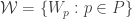
A collection of sets is said to be point-countable if every point in the space belongs to at most countably many sets in the collection. A base $\mathcal{G}$ for a space $X$ is said to be a point-countable base if $\mathcal{G}$ , in addition to being a base for the space $X$ , is also a point-countable collection of sets. The Michael line is an example of a space that has a point-countable base and that is not metrizable. The following is a point-countable base for $\mathbb{M}$ :

$\mathcal{G}=\mathcal{H} \cup \left\{\left\{ x \right\}: x \in \mathbb{P}\right\}$

where $\mathcal{H}$ is the set of all Euclidean open intervals with rational endpoints. One reason for the interest in point-countable base is that any countable compact space (hence any compact space) with a point-countable base is metrizable (see Metrization Theorems for Compact Spaces).

___________________________________________________________________________________

Reference

Engelking, R., General Topology, Revised and Completed edition, Heldermann Verlag, Berlin, 1989.
Willard, S., General Topology, Addison-Wesley Publishing Company, 1970.

___________________________________________________________________________________

$\copyright \ \ 2012$

Sorgenfrey Line is not a Moore Space

Posted on September 18, 2012 by Dan Ma

We found an incorrect statement about the Sorgenfrey line in an entry in Wikipedia about Moore space (link). This statement opens up a discussion on the question of whether the Sorgenfrey line is a Moore space as well as a discussion on Moore space. The following is the incorrect statement found in Wikipedia by the author.

5. Neither the Sorgenfrey line nor the Sorgenfrey plane are Moore spaces because they are normal and not second countable

The Sorgenfrey line is the space whose underlying set is the real line $S=\mathbb{R}$ where the topology is generated by a base consisting the half open intervals of the form $[a,b)$ . The Sorgenfrey plane is the square $S \times S$ .

Even though the Sorgenfrey line is normal, the Sorgenfrey plane is not normal. In fact, the Sorgenfrey line is the classic example of a normal space whose square is not normal. Both the Sorgenfrey line and the Sorgenfrey plane are not Moore space but not for the reason given. The statement seems to suggest that any normal Moore space is second countable. But this flies in the face of all the profound mathematics surrounding the normal Moore space conjecture, which is also discussed in the Wikipedia entry.

The statement indicated above is only a lead-in to a discussion of Moore space. We are certain that it will be corrected. We always appreciate readers who kindly alert us to errors found in this blog.

______________________________________________________________________________

Moore Spaces

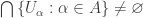
Let $X$ be a regular space. A development for $X$ is a sequence $\mathcal{G}_1,\mathcal{G}_2,\mathcal{G}_3,\cdots$ of open covers of $X$ such that for each $x \in X$ , and for each open subset $U$ of $X$ with $x \in U$ , there exists one cover $\mathcal{G}_n$ satisfying the condition that for any open set $V \in \mathcal{G}_n$ , $x \in V \Rightarrow V \subset U$ . When $X$ has a development, $X$ is said to be a Moore space (also called developable space). A Note On The Sorgenfrey Line is an introductory note on the Sorgenfrey line.

Moore spaces can be viewed as a generalization of metrizable spaces. Moore spaces are first countable (having a countable base at each point). For a development $\mathcal{G}_1,\mathcal{G}_2,\mathcal{G}_3,\cdots$ , the open sets in $\mathcal{G}_n$ are considered “smaller” as the index $n$ increases. In fact, this is how a development is defined for a metric space, where $\mathcal{G}_n$ consists of all open balls with diameters less than $\frac{1}{n}$ . Thus metric spaces are developable. There are plenty of non-metrizable Moore space. One example is the Niemytzki’s Tangent Disc space.

In a Moore space, every closed set is a $G_\delta$ -set. Thus if a Moore space is normal, it is perfectly normal. Any Moore space has a $G_\delta$ -diagonal (the diagonal $\Delta=\left\{(x,x): x \in X \right\}$ is a $G_\delta$ -set in $X \times X$ ). It is a well known theorem that every compact space with a $G_\delta$ -diagonal is metrizable. Thus any compact Moore space is metrizable.

The last statement can be shown more directly. Suppose that $X$ is compact and has a development $\mathcal{G}_1,\mathcal{G}_2,\mathcal{G}_3,\cdots$ . Then each $\mathcal{G}_n$ has a finite subcover $\mathcal{H}_n$ . Then $\bigcup_{n=1}^\infty \mathcal{H}_n$ is a countable base for $X$ . Thus any compact Moore space is second countable and hence metrizable.

What about paracompact Moore space? Suppose that $X$ is paracompact and has a development $\mathcal{G}_1,\mathcal{G}_2,\mathcal{G}_3,\cdots$ . Then each $\mathcal{G}_n$ has a locally finite open refinement $\mathcal{H}_n$ . Then $\bigcup_{n=1}^\infty \mathcal{H}_n$ is a $\sigma$ -locally finite base for $X$ . The Smirnov-Nagata metrization theorem states that a space is metrizable if and only if it has a $\sigma$ -locally finite base (see Theorem 23.9 on page 170 of [2]). Thus any paracompact Moore space has a $\sigma$ -locally finite base and is thus metrizable (after using the big gun of the Smirnov-Nagata metrization theorem).

______________________________________________________________________________

Sorgenfrey Line

The Sorgenfrey line is regular and Lindelof. Hence it is paracompact. Since the Sorgenfrey line is not metrizable, by the above discussion it cannot be a Moore space. The Sorgenfrey plane is also not a Moore space. Note that being a Moore space is a hereditary property. So if the Sorgenfrey plane is a Moore space, then every subspace of the Sorgenfrey plane (including the Sorgenfrey line) is a Moore space.

The following theorem is another way to show that the Sorgenfrey line is not a Moore space.

Bing’s Metrization Theorem

Every paracompact space is collectionwise normal (see Theorem 5.1.18, p.305 of [1]). Thus the Sorgenfrey line is collectionwise normal and hence cannot be a Moore space. A space $X$ is said to be collectionwise normal if $X$ is a $T_1$ -space and for every discrete collection $\left\{W_\alpha: \alpha \in A \right\}$ of closed sets in $X$ , there exists a discrete collection $\left\{V_\alpha: \alpha \in A \right\}$ of open subsets of $X$ such that $W_\alpha \subset V_\alpha$ . For a proof of Bing’s metrization theorem, see page 329 of [1].

______________________________________________________________________________

Remark

The normal Moore space conjecture is the statement that every normal Moore space is metrizable. This conjecture had been one of the key motivating questions for many set theorists and topologists during a large part of the twentieth century. The bottom line is that this statement cannot not be decided just on the basis of the set of generally accepted axioms called Zermelo–Fraenkel set theory with the axiom of choice, commonly abbreviated ZFC. But Bing’s metrization theorem states that if we strengthen normality to collectionwise normality, we have a definite answer.

______________________________________________________________________________

Reference

Engelking, R., General Topology, Revised and Completed edition, Heldermann Verlag, Berlin, 1989.
Willard, S., General Topology, Addison-Wesley Publishing Company, 1970.

______________________________________________________________________________

On Spaces That Can Never Be Dowker

Posted on December 6, 2009 by Dan Ma

A Dowker space is a normal space $X$ for which the product with the closed unit interval $[0,1]$ is not normal. In 1951, Dowker characterized Dowker’s spaces as those spaces that are normal but not countably paracompact ([1]). Soon after, spaces that are normal but not countably paracompact became known as Dowker spaces. In 1971, M. E. Rudin ([2]) constructed a ZFC example of a Dowker’s space. But this Dowker’s space is large. It has cardinality $(\omega_\omega)^\omega$ and is pathological in many ways. Thus the search for “nice” Dowker’s spaces continued. The Dowker’s spaces being sought were those with additional properties such as having various cardinal functions (e.g. density, character and weight) countable. Many “nice” Dowker’s spaces had been constructed using various additional set-theoretic assumptions. In 1996, Balogh constructed a first “small” Dowker’s space (cardinaltiy continuum) without additional set-theoretic axioms beyond ZFC ([4]). Rudin’s survey article is an excellent reference for Dowker’s spaces ([3]).

In this note, I make several additional observations on Dowker’s spaces. In this previous post, I presented a proof of the Dowker’s theorem characterizing the normal spaces for which the product with the unit interval is normal (see the statement of the Dowker’s theorem below). In another post, I showed that perfectly normal spaces can never be Dowker’s spaces. Based on the Dowker’s theorem, several other classes of spaces are easily seen as not Dowker.

Dowker’s Theorem. For a normal space $X$ , the following conditions are equivalent.

The space $X$ is countably paracompact.
The product $X \times Y$ is normal for any infinite compact metric space $Y$ .
The product $X \times [0,1]$ is normal.
For each sequence of closed subsets $\lbrace{A_0,A_1,A_2,...}\rbrace$ of $X$ such that $A_0 \supset A_1 \supset A_2 \supset ...$ and $\bigcap_{n<\omega} A_n=\phi$ , there is open sets $U_n \supset A_n$ for each $n$ such that $\bigcap_{n<\omega} U_n=\phi$ .

Observations. If $X$ is perfectly compact, then it can be shown that it is countably paracompact by showing that it satisfies condition 4 in the Dowker’s theorem (there is a proof in this blog). Thus there are no perfectly normal Dowker’s spaces. There are no countably compact Dowker’s spaces since any countably compact space is countably paracompact. This can also be seen using condition 4 above. In a countably compact space, any decreasing nested sequence of closed sets has non-empty intersection and thus condition 4 is satisfied vacuously. Furthermore, all metric spaces, compact spaces, regular Lindelof spaces cannot be Dowker since these spaces are paracomapct.

Normal Moore spaces are perfectly normal. Thus there are no Dowker’s spaces that are Moore spaces. Note that a space is perfectly normal if it is normal and if every closed set is $G_\delta$ . We show that in a Moore space, every closed set is $G_\delta$ . Let $\lbrace{\mathcal{O}_n:n \in \omega}\rbrace$ be a development for the regular space $X$ . Let $A$ be a closed set in $X$ . We show that $A$ is a $G_\delta-$ set in $X$ . For each $n$ , let $U_n=\lbrace{O \in \mathcal{O}_n:O \bigcap A \neq \phi}\rbrace$ . Obviously, $A \subset \bigcap_n U_n$ . Let $x \in \bigcap_n U_n$ . If $x \notin A$ , there is some $n$ such that for each $O \in \mathcal{O}_n$ with $x \in O$ , we have $O \subset X-A$ . Since $x \in \bigcap_n U_n$ , $x \in O$ for some $O \in \mathcal{O}_n$ and $O \cap A \neq \phi$ , a contradiction. Thus we have $A=\bigcap_n U_n$ .

There are other classes of spaces that can never be Dowker. We point these out without proof. For example, there are no linearly ordered Dowker’s spaces and there are no monotonically normal Dowker’s spaces (see Rudin’s survey article [3]).

Reference

Dowker, C. H., On Countably Paracompact Spaces, Canad. J. Math. 3, (1951) 219-224.
Rudin, M. E., A normal space $X$ for which $X \times I$ is not normal, Fund. Math., 73 (1971), 179-186.
Rudin, M. E., Dowker Spaces, Handbook of Set-Theoretic Topology (K. Kunen and J. E. Vaughan, eds), Elsevier Science Publishers B. V., Amsterdam, (1984) 761-780.
Balogh, Z., A small Dowker space in ZFC, Proc. Amer. Math. Soc., 124 (1996), 2555-2560.

A Note About Countably Compact Spaces

Posted on December 2, 2009 by Dan Ma

This is a discussion on several additional conditions that would turn a countably compact space into a compact space. For example, a countably compact space having a $G_\delta-$ diagonal is compact (proved in this post). Each of the following properties, if possessed by a countably compact space, would lead to compactness: (1) having a $G_\delta-$ diagonal, (2) being metrizable, (3) being a Moore space, (4) being paracompact, and (5) being metacompact. All spaces are at least Hausdorff. We have the following theorem. Some relevant definitions and links to posts in this blog are given below. For any terms that are not defined here, see Engelking ([1]).

Theorem. Let $X$ be a countably compact space. If $X$ possesses any one of the following conditions, then $X$ is compact.

Having a $G_\delta-$ diagonal.
Being a metrizable space.
Being a Moore space.
Being a paracompact space.
Being a metacompact space.

The proof of 1 has already been presented in another post in this blog. Since metrizable spaces are Moore spaces, between 2 and 3 we only need to prove 3. Between 4 and 5, we only need to prove 5 (since paracompact compact spaces are metacompact).

Proof of 3. A Moore space is a regular space that has a development (see this post for the definition). In this post, I showed that a space $X$ has a $G_\delta-$ diagonal if and only it has a $G_\delta-$ diagonal sequence. It is easy to verify that the development for a Moore space is a $G_\delta-$ diagonal sequence. Thus any Moore space has a $G_\delta-$ diagonal and any countably compact Moore space is compact (and metrizable). Saying in another way, in the class of Moore spaces, countably compactness is equivalent to compactness.

Proof of 5. A space $X$ is metacompact if every open cover of $X$ has a point-finite open refinement. Let $X$ be metacompact. Let $\mathcal{U}$ be an open cover of $X$ . By the metacompactness, $\mathcal{U}$ has a point-finite open refinement $\mathcal{O}$ . We are done if we can show $\mathcal{O}$ has a finite subcover. This finite subcover is obtained through the following claims.

Claim 1. There is a set $M \subset X$ such that $\lvert M \cap O \lvert \thinspace \leq 1$ for each $O \in \mathcal{O}$ and such that $M$ is maximal. That is, by adding an additional point $x \notin M$ , $\lvert (M \cup \lbrace{x}\rbrace) \cap O \lvert \thinspace \ge 2$ for some $O \in \mathcal{O}$ .

Such a set can be obtained by using the Zorn’s Lemma.

Claim 2. Let $\mathcal{W}=\lbrace{O \in \mathcal{O}:O \cap M \neq \phi}\rbrace$ . We claim that $\mathcal{W}$ is an open cover of $X$ .

To see this, let $x \in X$ . If $x \in M$ , then $x \in O$ for some $O \in \mathcal{W}$ . If $x \notin M$ , then by the maximality of $M$ , $M \cup \lbrace{x}\rbrace$ intersects with some $O \in \mathcal{O}$ with at least 2 points. This means that $x$ and at least one point of $M$ are in $O$ . Then $O \in \mathcal{W}$ .

Since each open set in $\mathcal{W}$ contains at most one point of $M$ , $M$ is a closed and discrete set in $X$ . By the countably compactness of $X$ , $M$ must be finite. Since each point of $M$ is in at most finitely many open sets in $\mathcal{O}$ , $\mathcal{W}$ is finite. Thus $\mathcal{W}$ is a finite subcover of $\mathcal{O}$ .

Reference

Engelking, R., General Topology, Revised and Completed Edition, 1989, Heldermann Verlag, Berlin.

Network Weight of Topological Spaces – II

Posted on November 17, 2009 by Dan Ma

This is a continuation of the discussion on network. In the previous post, I showed that the network weight (the minimum cardinality of a network) coincides with the weight for both metrizable spaces and locally compact spaces. In another post, I showed that this is true for compact spaces. I now show that this is also true for the class of Moore spaces. First, some definitions. A sequence $\lbrace{\mathcal{D}_n}\rbrace_{n<\omega}$ of open covers of a space $X$ is a development for $X$ if for each $x \in X$ and each open set $U \subset X$ with $x \in U$ , there is some $n$ such that any open set in $\mathcal{D}_n$ containing the point $x$ is contained in $U$ . A developable space is one that has a development. A Moore space is a regular developable space.

For a collection of $\mathcal{G}$ of subsets of a space $X$ and for $x \in X$ , define $st(x,\mathcal{G})=\bigcup\lbrace{U \in \mathcal{G}:x \in U}\rbrace$ . An equivalent way of defining a development: A sequence $\lbrace{\mathcal{D}_n}\rbrace_{n<\omega}$ of open covers of a space $X$ is a development for $X$ if for each $x \in X$ , $\lbrace{st(x,\mathcal{G}_n):n \in \omega}\rbrace$ is a local base at $x$ . For a basic introduction to Moore space and the Moore space conjecture, there are numerous places to look in the literature ([1] being one of them).

Theorem. If $X$ is a Moore space, then $nw(X)=w(X)$ .

Proof. Since $nw(X) \leq w(X)$ always holds, we only need to show $w(X) \leq nw(X)$ . To this end, we exhibit a base $\mathcal{B}$ with $\vert \mathcal{B} \lvert \leq nw(X)$ . Let $\lbrace{\mathcal{D}_n}\rbrace_{n<\omega}$ be a development for $X$ . Let $\mathcal{N}$ be a network with cardinality $nw(X)$ .

For each $N \in \mathcal{N}$ , choose open set $O(n,N) \in \mathcal{D}_n$ such that $N \subset O(n,N)$ . Let $\mathcal{B}_n=\lbrace{O(n,N):N \in \mathcal{N}}\rbrace$ and $\mathcal{B}=\bigcup_{n<\omega}\mathcal{B}_n$ . Note that $\lvert \mathcal{B} \lvert \leq nw(X)$ . Because $\mathcal{N}$ is a network, each $\mathcal{B}_n$ is a cover of $X$ . To see this, let $x \in X$ . Choose some $V \in \mathcal{D}_n$ such that $x \in V$ . There is some $N \in \mathcal{N}$ such that $x \in N \subset V$ . Then $x \in O(n,N)$ . For each $n$ , $\mathcal{B}_n \subset \mathcal{D}_n$ . The sequence $\lbrace{\mathcal{B}_n}\rbrace$ works like a development. We have just shown that $\mathcal{B}$ is a base for $X$ .

Corollary. The example of Butterfly space is not a Moore space.

The example of the Butterfly (or Bow-tie) space is defined in this previous post. This space has a countable network and the weight of this space is continuum. Thus this space cannot be a Moore space.

Reference
[1] Steen, L. A. & Seebach, J. A. [1995] Counterexamples in Topology, Dover Books.

Dan Ma's Topology Blog

Expository Articles In General Topology

Category Archives: Moore space

Bing’s Example G

Michael Line Basics

Sorgenfrey Line is not a Moore Space

On Spaces That Can Never Be Dowker

A Note About Countably Compact Spaces

Network Weight of Topological Spaces – II